Data quality control

Sequencing technologies all have some amount of error. Some of this error happens during PCR and some happens during sequencing. There are lots of ways to filter out errors including:

Removing sequences/bases that the sequencer indicates are low quality. This information is typically in the .fastq files returned by the sequencer. There are many programs, such as trimmomatic, that can use the quality scores in these files to filter out low-quality sequences.
Clustering similar sequences together. Many erroneous sequences are very similar to the true sequences, so they will be incorporated into the same OTU as the true sequence. In that sense, clustering into OTUs will hide some sequencing error.
Removal of chimeric sequences. “Chimeras” are more significant errors that occur during PCR when an incomplete amplicon acts as a primer for a different template in a subsequent cycle. Most amplicon metagenomic pipelines (e.g. QIIME, mothur, usearch) have functions to detect and remove chimeras.
Removing low-abundance sequences. Most of the time, erroneous sequences will occur much less often than the true sequence. Simply removing any unique sequence / OTU that appears less than some minimum number of times is an effective way to remove these errors. OTUs represented by only a single sequence are commonly called singletons. So when you hear things like “singletons were removed” and means all OTUs composed of only a single sequence were removed.
Rarefying read counts. Usually, we try to make each sample in a sequencing run have the same number of reads sequenced, but that does not always happen. When a sample has many more reads than another sample, its apparent diversity can be artificially inflated since rare taxa are more likely to be found. To avoid this, the reads are subsampled to a fixed number or “rarefied”. This technique can throw out a lot of data, so it is not always appropriate (McMurdie and Holmes (2014)).
Converting counts to presence/absence. Due to PCR biases and the nature of compositional data, many researchers advocate not using read count information at all. Instead, they recommend converting counts to simply “present” or “absent”.

Since we are only working with abundance matrices in these tutorials, the first three types of quality control have already been done (ideally), but we can still remove low-abundance OTUs and rarefy the counts of the remaining OTUs.

Load example data

If you are starting the workshop at this section, or had problems running code in a previous section, use the following to load the data used in this section. You can download the “filtered_data.Rdata” file here. If obj and sample_data are already in your environment, you can ignore this and proceed.

load("filtered_data.Rdata")

Removing low-abundance counts

The easiest way to get rid of some error in your data is to throw out any count information below some threshold. The threshold is up to you; removing singletons or doubletons is common, but lets be more conservative and remove any counts less than 10. The zero_low_counts counts can be used to convert any counts less than some number to zero.

library(metacoder)
obj$data$otu_counts <- zero_low_counts(obj, "otu_counts", min_count = 10,
                                       other_cols = TRUE) # keep OTU_ID column

## No `cols` specified, so using all numeric columns:
##    M1981P563, M1977P1709, M1980P502, M1981P606 ... M1955P747, M1978P342, M1955P778

## Zeroing 576512 of 6331728 counts less than 10.

print(obj)

## <Taxmap>
##   704 taxa: aad. Bacteria, aaf. Proteobacteria ... cgz. S24-7, chs. Alcanivoracaceae
##   704 edges: NA->aad, aad->aaf, aad->aag, aad->aah ... amg->cgf, arh->cgz, apt->chs
##   1 data sets:
##     otu_counts:
##       # A tibble: 21,684 × 294
##         taxon_id OTU_ID M1981P563 M1977P…¹ M1980…² M1981…³ M1981…⁴ M1981…⁵ M1981…⁶ M1982…⁷
##         <chr>    <chr>      <dbl>    <dbl>   <dbl>   <dbl>   <dbl>   <dbl>   <dbl>   <dbl>
##       1 ben      2              0        0       0       0       0       0      24       0
##       2 beo      3          10251       59   15857     309     134      90   11391      63
##       3 ben      4           1447     2496    2421    3331     143    1847    2120    2048
##       # … with 21,681 more rows, 284 more variables: M1979P447 <dbl>, M1982P701 <dbl>,
##       #   M1982P661 <dbl>, M1978P293 <dbl>, M1980P462 <dbl>, M1555P221 <dbl>,
##       #   M1980P471 <dbl>, M1979P422 <dbl>, M1982P655 <dbl>, M1554P182 <dbl>, …, and
##       #   abbreviated variable names ¹M1977P1709, ²M1980P502, ³M1981P606, ⁴M1981P599,
##       #   ⁵M1981P611, ⁶M1981P587, ⁷M1982P729
##   0 functions:

That set all read counts less than 10 to zero. It did not filter out any OTUs or their associated taxa however. We can do that using filter_obs, which is used to filter data associated with a taxonomy in a taxmap object. First lets find which OTUs now have now reads associated with them.

no_reads <- rowSums(obj$data$otu_counts[, sample_data$SampleID]) == 0
sum(no_reads) # when `sum` is used on a TRUE/FALSE vector it counts TRUEs

## [1] 14990

So now 14,990 of 21,684 OTUs have no reads. We can remove them and the taxa they are associated with like so:

obj <- filter_obs(obj, "otu_counts", ! no_reads, drop_taxa = TRUE)
print(obj)

## <Taxmap>
##   489 taxa: aad. Bacteria, aaf. Proteobacteria ... ccz. Enterococcaceae, cfp. Dermacoccaceae
##   489 edges: NA->aad, aad->aaf, aad->aag, aad->aah ... amj->byk, aqy->ccz, amj->cfp
##   1 data sets:
##     otu_counts:
##       # A tibble: 6,694 × 294
##         taxon_id OTU_ID M1981P563 M1977P…¹ M1980…² M1981…³ M1981…⁴ M1981…⁵ M1981…⁶ M1982…⁷
##         <chr>    <chr>      <dbl>    <dbl>   <dbl>   <dbl>   <dbl>   <dbl>   <dbl>   <dbl>
##       1 ben      2              0        0       0       0       0       0      24       0
##       2 beo      3          10251       59   15857     309     134      90   11391      63
##       3 ben      4           1447     2496    2421    3331     143    1847    2120    2048
##       # … with 6,691 more rows, 284 more variables: M1979P447 <dbl>, M1982P701 <dbl>,
##       #   M1982P661 <dbl>, M1978P293 <dbl>, M1980P462 <dbl>, M1555P221 <dbl>,
##       #   M1980P471 <dbl>, M1979P422 <dbl>, M1982P655 <dbl>, M1554P182 <dbl>, …, and
##       #   abbreviated variable names ¹M1977P1709, ²M1980P502, ³M1981P606, ⁴M1981P599,
##       #   ⁵M1981P611, ⁶M1981P587, ⁷M1982P729
##   0 functions:

Rarefaction

Rarefaction is used to simulate even numbers of reads per sample. Even sampling is important for at least two reasons:

When comparing diversity of samples, more samples make it more likely to observe rare species. This will have a larger effect on some diversity indexes than others, depending on how they weigh rare species.
When comparing the similarity of samples, the presence of rare species due to higher sampling depth in one sample but not another can make the two samples appear more different than they actually are.

Therefore, when comparing the diversity or similarity of samples, it is important to take into account differences in sampling depth.

Rarefying can waste a lot of data and is not needed in many cases. See McMurdie and Holmes (2014) for an in-depth discussion on alternatives to rarefaction. We cover it here because it is a popular technique.

Typically, the rarefaction depth chosen is the minimum sample depth. If the minimum depth is very small, the samples with the smallest depth can be removed and the minimum depth of the remaining samples can be used.

Lets take a look at the distribution of read depths of our samples:

hist(colSums(obj$data$otu_counts[, sample_data$SampleID]))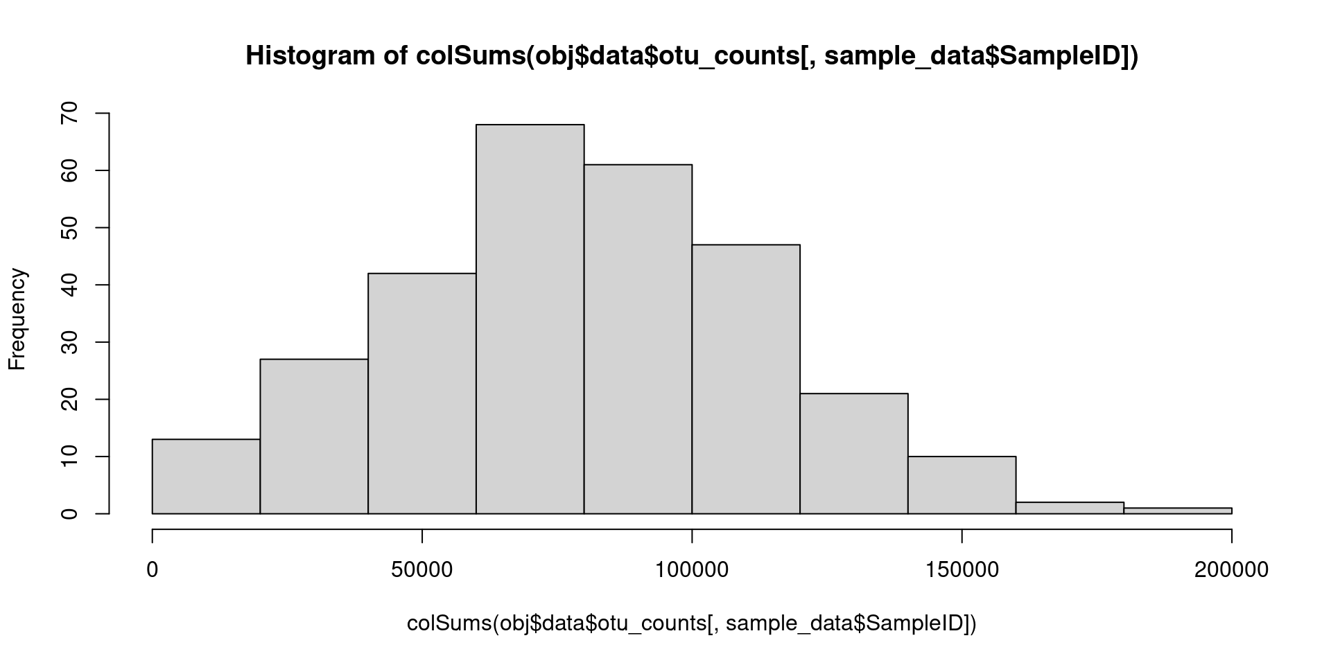

We have a minimum depth of 1857, a median of 78767 and a maximum depth of 1.89353^{5}. We could try to remove one or two of the samples with the smallest depth, since it seems like a waste to throw out so much data, but for this tutorial we will just rarefy to the minimum of 1857 reads. The vegan package implements many functions to help with rarefying data, but we will use a function from metacoder that calls the functions from vegan and re-formats the input and outputs to make them easier to use with the way our data is formatted.

obj$data$otu_rarefied <- rarefy_obs(obj, "otu_counts", other_cols = TRUE)

## No `cols` specified, so using all numeric columns:
##    M1981P563, M1977P1709, M1980P502, M1981P606 ... M1955P747, M1978P342, M1955P778

## Rarefying to 1857 since that is the lowest sample total.

print(obj)

## <Taxmap>
##   489 taxa: aad. Bacteria, aaf. Proteobacteria ... ccz. Enterococcaceae, cfp. Dermacoccaceae
##   489 edges: NA->aad, aad->aaf, aad->aag, aad->aah ... amj->byk, aqy->ccz, amj->cfp
##   2 data sets:
##     otu_counts:
##       # A tibble: 6,694 × 294
##         taxon_id OTU_ID M1981P563 M1977P…¹ M1980…² M1981…³ M1981…⁴ M1981…⁵ M1981…⁶ M1982…⁷
##         <chr>    <chr>      <dbl>    <dbl>   <dbl>   <dbl>   <dbl>   <dbl>   <dbl>   <dbl>
##       1 ben      2              0        0       0       0       0       0      24       0
##       2 beo      3          10251       59   15857     309     134      90   11391      63
##       3 ben      4           1447     2496    2421    3331     143    1847    2120    2048
##       # … with 6,691 more rows, 284 more variables: M1979P447 <dbl>, M1982P701 <dbl>,
##       #   M1982P661 <dbl>, M1978P293 <dbl>, M1980P462 <dbl>, M1555P221 <dbl>,
##       #   M1980P471 <dbl>, M1979P422 <dbl>, M1982P655 <dbl>, M1554P182 <dbl>, …, and
##       #   abbreviated variable names ¹M1977P1709, ²M1980P502, ³M1981P606, ⁴M1981P599,
##       #   ⁵M1981P611, ⁶M1981P587, ⁷M1982P729
##     otu_rarefied:
##       # A tibble: 6,694 × 294
##         taxon_id OTU_ID M1981P563 M1977P…¹ M1980…² M1981…³ M1981…⁴ M1981…⁵ M1981…⁶ M1982…⁷
##         <chr>    <chr>      <dbl>    <dbl>   <dbl>   <dbl>   <dbl>   <dbl>   <dbl>   <dbl>
##       1 ben      2              0        0       0       0       0       0       1       0
##       2 beo      3            402        4     428       5     134       0     347       2
##       3 ben      4             63       46      67      77     143      50      70      44
##       # … with 6,691 more rows, 284 more variables: M1979P447 <dbl>, M1982P701 <dbl>,
##       #   M1982P661 <dbl>, M1978P293 <dbl>, M1980P462 <dbl>, M1555P221 <dbl>,
##       #   M1980P471 <dbl>, M1979P422 <dbl>, M1982P655 <dbl>, M1554P182 <dbl>, …, and
##       #   abbreviated variable names ¹M1977P1709, ²M1980P502, ³M1981P606, ⁴M1981P599,
##       #   ⁵M1981P611, ⁶M1981P587, ⁷M1982P729
##   0 functions:

This probably means that some OTUs now have no reads in the rarefied dataset. Lets remove those like we did before. However, since there is now two tables, we should not remove any taxa since they still might be used in the rarefied table, so we will not add the drop_taxa = TRUE option this time.

no_reads <- rowSums(obj$data$otu_rarefied[, sample_data$SampleID]) == 0
obj <- filter_obs(obj, "otu_rarefied", ! no_reads)
print(obj)

## <Taxmap>
##   489 taxa: aad. Bacteria, aaf. Proteobacteria ... ccz. Enterococcaceae, cfp. Dermacoccaceae
##   489 edges: NA->aad, aad->aaf, aad->aag, aad->aah ... amj->byk, aqy->ccz, amj->cfp
##   2 data sets:
##     otu_counts:
##       # A tibble: 6,694 × 294
##         taxon_id OTU_ID M1981P563 M1977P…¹ M1980…² M1981…³ M1981…⁴ M1981…⁵ M1981…⁶ M1982…⁷
##         <chr>    <chr>      <dbl>    <dbl>   <dbl>   <dbl>   <dbl>   <dbl>   <dbl>   <dbl>
##       1 ben      2              0        0       0       0       0       0      24       0
##       2 beo      3          10251       59   15857     309     134      90   11391      63
##       3 ben      4           1447     2496    2421    3331     143    1847    2120    2048
##       # … with 6,691 more rows, 284 more variables: M1979P447 <dbl>, M1982P701 <dbl>,
##       #   M1982P661 <dbl>, M1978P293 <dbl>, M1980P462 <dbl>, M1555P221 <dbl>,
##       #   M1980P471 <dbl>, M1979P422 <dbl>, M1982P655 <dbl>, M1554P182 <dbl>, …, and
##       #   abbreviated variable names ¹M1977P1709, ²M1980P502, ³M1981P606, ⁴M1981P599,
##       #   ⁵M1981P611, ⁶M1981P587, ⁷M1982P729
##     otu_rarefied:
##       # A tibble: 5,025 × 294
##         taxon_id OTU_ID M1981P563 M1977P…¹ M1980…² M1981…³ M1981…⁴ M1981…⁵ M1981…⁶ M1982…⁷
##         <chr>    <chr>      <dbl>    <dbl>   <dbl>   <dbl>   <dbl>   <dbl>   <dbl>   <dbl>
##       1 ben      2              0        0       0       0       0       0       1       0
##       2 beo      3            402        4     428       5     134       0     347       2
##       3 ben      4             63       46      67      77     143      50      70      44
##       # … with 5,022 more rows, 284 more variables: M1979P447 <dbl>, M1982P701 <dbl>,
##       #   M1982P661 <dbl>, M1978P293 <dbl>, M1980P462 <dbl>, M1555P221 <dbl>,
##       #   M1980P471 <dbl>, M1979P422 <dbl>, M1982P655 <dbl>, M1554P182 <dbl>, …, and
##       #   abbreviated variable names ¹M1977P1709, ²M1980P502, ³M1981P606, ⁴M1981P599,
##       #   ⁵M1981P611, ⁶M1981P587, ⁷M1982P729
##   0 functions:

Proportions

An easy alternative to rarefaction is to convert read counts to proportions of reads per-sample. This makes samples directly comparable, but does not solve the problem with inflated diversity estimates discussed in the rarefaction section. See McMurdie and Holmes (2014) for an in-depth discussion on the relative merits of proportions, rarefaction, and other (better) methods.

To convert counts to proportions in metacoder, we can use the calc_obs_props function:

obj$data$otu_props <- calc_obs_props(obj, "otu_counts", other_cols = TRUE)

## No `cols` specified, so using all numeric columns:
##    M1981P563, M1977P1709, M1980P502, M1981P606 ... M1955P747, M1978P342, M1955P778

## Calculating proportions from counts for 292 columns for 6694 observations.

print(obj)

## <Taxmap>
##   489 taxa: aad. Bacteria, aaf. Proteobacteria ... ccz. Enterococcaceae, cfp. Dermacoccaceae
##   489 edges: NA->aad, aad->aaf, aad->aag, aad->aah ... amj->byk, aqy->ccz, amj->cfp
##   3 data sets:
##     otu_counts:
##       # A tibble: 6,694 × 294
##         taxon_id OTU_ID M1981P563 M1977P…¹ M1980…² M1981…³ M1981…⁴ M1981…⁵ M1981…⁶ M1982…⁷
##         <chr>    <chr>      <dbl>    <dbl>   <dbl>   <dbl>   <dbl>   <dbl>   <dbl>   <dbl>
##       1 ben      2              0        0       0       0       0       0      24       0
##       2 beo      3          10251       59   15857     309     134      90   11391      63
##       3 ben      4           1447     2496    2421    3331     143    1847    2120    2048
##       # … with 6,691 more rows, 284 more variables: M1979P447 <dbl>, M1982P701 <dbl>,
##       #   M1982P661 <dbl>, M1978P293 <dbl>, M1980P462 <dbl>, M1555P221 <dbl>,
##       #   M1980P471 <dbl>, M1979P422 <dbl>, M1982P655 <dbl>, M1554P182 <dbl>, …, and
##       #   abbreviated variable names ¹M1977P1709, ²M1980P502, ³M1981P606, ⁴M1981P599,
##       #   ⁵M1981P611, ⁶M1981P587, ⁷M1982P729
##     otu_rarefied:
##       # A tibble: 5,025 × 294
##         taxon_id OTU_ID M1981P563 M1977P…¹ M1980…² M1981…³ M1981…⁴ M1981…⁵ M1981…⁶ M1982…⁷
##         <chr>    <chr>      <dbl>    <dbl>   <dbl>   <dbl>   <dbl>   <dbl>   <dbl>   <dbl>
##       1 ben      2              0        0       0       0       0       0       1       0
##       2 beo      3            402        4     428       5     134       0     347       2
##       3 ben      4             63       46      67      77     143      50      70      44
##       # … with 5,022 more rows, 284 more variables: M1979P447 <dbl>, M1982P701 <dbl>,
##       #   M1982P661 <dbl>, M1978P293 <dbl>, M1980P462 <dbl>, M1555P221 <dbl>,
##       #   M1980P471 <dbl>, M1979P422 <dbl>, M1982P655 <dbl>, M1554P182 <dbl>, …, and
##       #   abbreviated variable names ¹M1977P1709, ²M1980P502, ³M1981P606, ⁴M1981P599,
##       #   ⁵M1981P611, ⁶M1981P587, ⁷M1982P729
##     otu_props:
##       # A tibble: 6,694 × 294
##         taxon_id OTU_ID M1981P563 M1977P…¹ M1980…² M1981…³ M1981…⁴ M1981…⁵ M1981…⁶ M1982…⁷
##         <chr>    <chr>      <dbl>    <dbl>   <dbl>   <dbl>   <dbl>   <dbl>   <dbl>   <dbl>
##       1 ben      2         0      0         0      0        0      0       4.09e-4 0      
##       2 beo      3         0.200  0.000448  0.237  0.00327  0.0722 0.00101 1.94e-1 6.68e-4
##       3 ben      4         0.0282 0.0189    0.0362 0.0352   0.0770 0.0207  3.61e-2 2.17e-2
##       # … with 6,691 more rows, 284 more variables: M1979P447 <dbl>, M1982P701 <dbl>,
##       #   M1982P661 <dbl>, M1978P293 <dbl>, M1980P462 <dbl>, M1555P221 <dbl>,
##       #   M1980P471 <dbl>, M1979P422 <dbl>, M1982P655 <dbl>, M1554P182 <dbl>, …, and
##       #   abbreviated variable names ¹M1977P1709, ²M1980P502, ³M1981P606, ⁴M1981P599,
##       #   ⁵M1981P611, ⁶M1981P587, ⁷M1982P729
##   0 functions:

Rarefaction curves

The relationship between the number of reads and the number of OTUs can be described using rarefaction curves. This is actually different concept than rarefaction, and it is done for different reasons. Rarefaction is a subsampling technique meant to correct for uneven sample size whereas rarefaction curves are used to estimate whether all the diveristy of the true community was captured.
Each line represents a different sample (i.e. column) and shows how many OTUs are found in a random subsets of different numbers of reads. The rarecurve function from the vegan package will do the random sub-sampling and plot the results for an abundance matrix. For example, the code below plots the rarefaction curve for a single sample:

library(vegan)

## Loading required package: permute

## Loading required package: lattice

## This is vegan 2.6-2

rarecurve(t(obj$data$otu_counts[, "M1981P563"]), step = 20,
          sample = min(colSums(obj$data$otu_counts[, sample_data$SampleID])),
          col = "blue", cex = 1.5)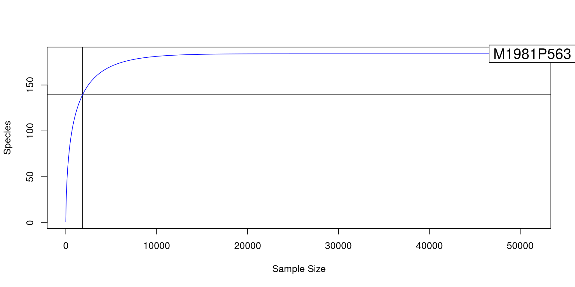

For this sample, few new OTUs are observed after about 20,000 reads. Since the number of OTUs found flattens out, it suggests that the sample had sufficient reads to capture most of the diversity (or reach a point of diminishing returns). 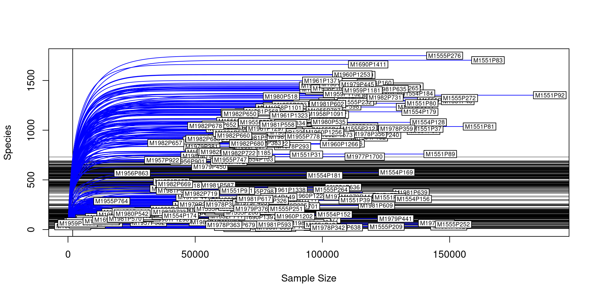Like other functions in vegan, rarecurve expects samples to in rows instead of columns, so we had to transpose (make rows columns) the matrix with the t function before passing it to rarecurve. If you plot all the samples, which takes a few minutes, it looks like this:

Converting to presence/absence

Many researchers believe that read depth is not informative due to PCR and sequencing biases. Therefore, instead of comparing read counts, the counts can be converted to presence or absence of an OTU in a given sample. This can be done like so:

counts_to_presence(obj, "otu_rarefied")

## No `cols` specified, so using all numeric columns:
##    M1981P563, M1977P1709, M1980P502, M1981P606 ... M1955P747, M1978P342, M1955P778

## # A tibble: 5,025 × 293
##    taxon_id M1981P…¹ M1977…² M1980…³ M1981…⁴ M1981…⁵ M1981…⁶ M1981…⁷ M1982…⁸ M1979…⁹ M1982…˟ M1982…˟
##    <chr>    <lgl>    <lgl>   <lgl>   <lgl>   <lgl>   <lgl>   <lgl>   <lgl>   <lgl>   <lgl>   <lgl>  
##  1 ben      FALSE    FALSE   FALSE   FALSE   FALSE   FALSE   TRUE    FALSE   FALSE   FALSE   TRUE   
##  2 beo      TRUE     TRUE    TRUE    TRUE    TRUE    FALSE   TRUE    TRUE    TRUE    TRUE    TRUE   
##  3 ben      TRUE     TRUE    TRUE    TRUE    TRUE    TRUE    TRUE    TRUE    TRUE    TRUE    TRUE   
##  4 bep      TRUE     TRUE    TRUE    TRUE    FALSE   TRUE    TRUE    TRUE    TRUE    TRUE    FALSE  
##  5 beq      TRUE     TRUE    TRUE    TRUE    FALSE   TRUE    TRUE    TRUE    TRUE    TRUE    FALSE  
##  6 amk      TRUE     TRUE    TRUE    TRUE    TRUE    TRUE    TRUE    TRUE    TRUE    TRUE    TRUE   
##  7 bes      FALSE    TRUE    FALSE   TRUE    FALSE   TRUE    TRUE    TRUE    TRUE    TRUE    FALSE  
##  8 bet      TRUE     TRUE    TRUE    TRUE    TRUE    FALSE   TRUE    FALSE   TRUE    TRUE    TRUE   
##  9 beu      TRUE     TRUE    TRUE    TRUE    FALSE   FALSE   TRUE    FALSE   TRUE    TRUE    FALSE  
## 10 bev      FALSE    TRUE    FALSE   TRUE    FALSE   TRUE    TRUE    TRUE    TRUE    TRUE    FALSE  
## # … with 5,015 more rows, 281 more variables: M1978P293 <lgl>, M1980P462 <lgl>, M1555P221 <lgl>,
## #   M1980P471 <lgl>, M1979P422 <lgl>, M1982P655 <lgl>, M1554P182 <lgl>, M1981P623 <lgl>,
## #   M1555P239 <lgl>, M1958P1020 <lgl>, …, and abbreviated variable names ¹M1981P563, ²M1977P1709,
## #   ³M1980P502, ⁴M1981P606, ⁵M1981P599, ⁶M1981P611, ⁷M1981P587, ⁸M1982P729, ⁹M1979P447, ˟M1982P701,
## #   ˟M1982P661

For this workshop however, we will use the read counts.

Exercises

In these exercises, we will be using the obj from the analysis above. If you did not run the code above or had problems, run the following code to get the objects used. You can download the “clean_data.Rdata” file here.

load("clean_data.Rdata")

1a) Consider the following rarefaction curves:

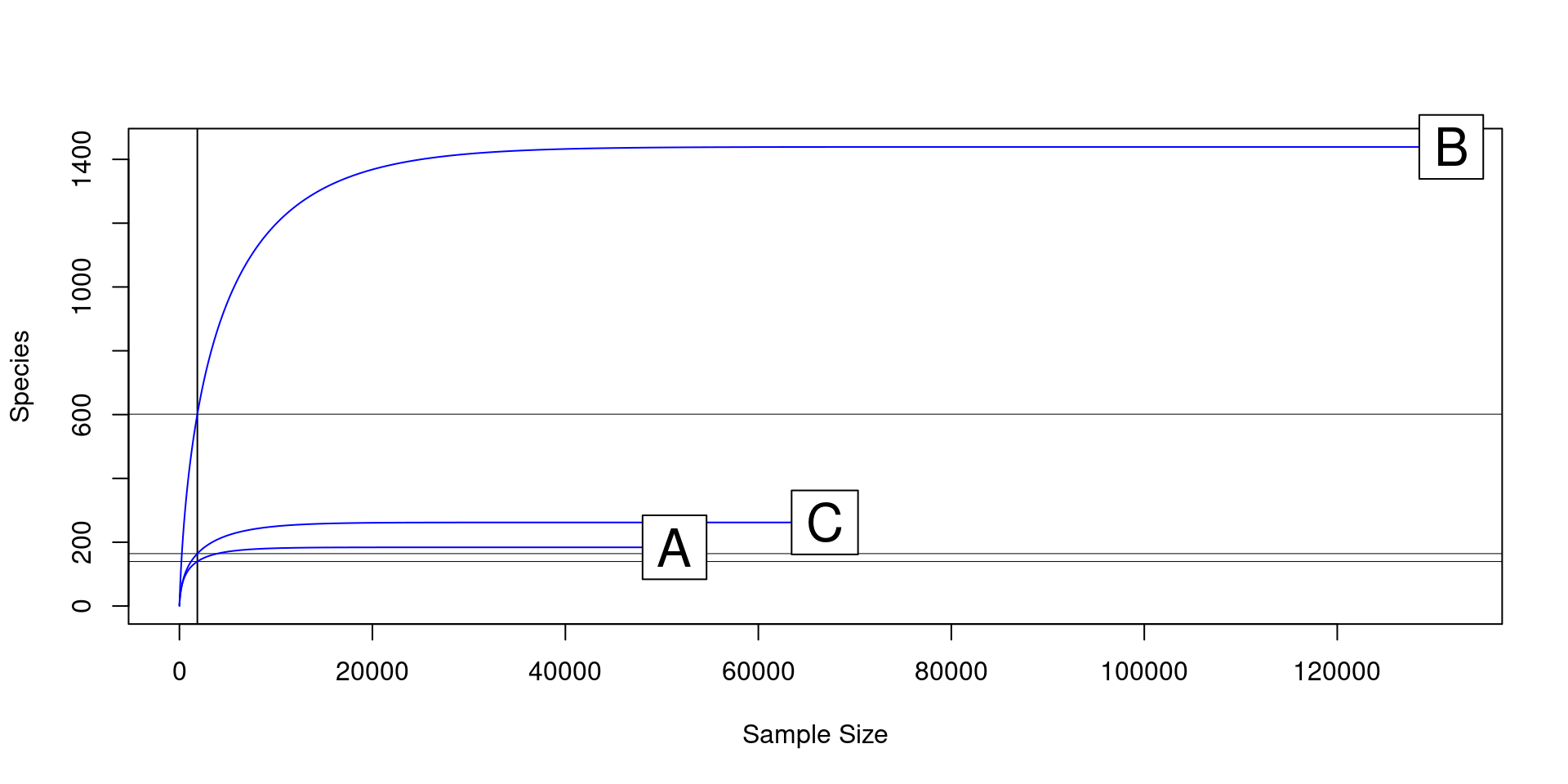
1b) Which sample is more diverse?

1c) Which sample needs the most reads to capture all of its diversity?

1d) What would be a sufficient read count to capture all of the diversity in these three samples?

Around 40,000 reads.

2) Look at the documentation for rarefy_obs. Rarefy the sample OTU counts to 1000 reads.

rarefy_obs(obj, "otu_counts", sample_size = 1000)

## No `cols` specified, so using all numeric columns:
##    M1981P563, M1977P1709, M1980P502, M1981P606 ... M1955P747, M1978P342, M1955P778

## # A tibble: 6,694 × 293
##    taxon_id M1981P…¹ M1977…² M1980…³ M1981…⁴ M1981…⁵ M1981…⁶ M1981…⁷ M1982…⁸ M1979…⁹ M1982…˟ M1982…˟
##    <chr>       <dbl>   <dbl>   <dbl>   <dbl>   <dbl>   <dbl>   <dbl>   <dbl>   <dbl>   <dbl>   <dbl>
##  1 ben             0       0       0       0       0       0       0       0       0       0      56
##  2 beo           202       0     241       3      72       2     187       0     137       6       3
##  3 ben            30      12      36      34      82      28      27      20      96      34     258
##  4 bep             3       3       6       8       0       6       5       5       5       1       0
##  5 beq             1      23       4      21       0      32       0      15       1      50       0
##  6 amk            40       2      83       9     115       2      63       2     229       8     411
##  7 bes             1      32       0      18       0      31       7      23       1      19       0
##  8 bet             2       1       1       0       8       0       5       0      36       1       1
##  9 beu            46       0      64       1       0       0      69       0       6       2       0
## 10 bev             4      18       0      24       0      24       0      33       1      10       0
## # … with 6,684 more rows, 281 more variables: M1978P293 <dbl>, M1980P462 <dbl>, M1555P221 <dbl>,
## #   M1980P471 <dbl>, M1979P422 <dbl>, M1982P655 <dbl>, M1554P182 <dbl>, M1981P623 <dbl>,
## #   M1555P239 <dbl>, M1958P1020 <dbl>, …, and abbreviated variable names ¹M1981P563, ²M1977P1709,
## #   ³M1980P502, ⁴M1981P606, ⁵M1981P599, ⁶M1981P611, ⁷M1981P587, ⁸M1982P729, ⁹M1979P447, ˟M1982P701,
## #   ˟M1982P661

3) What are two ways of accounting for uneven sample depth?

Rarefaction and converting counts to proportions.

4) What are some reasons that read counts might not correspond to species abundance in the original sample? Try to think of at least 3. There are 7 listed in the answer below and there are probably other reasons not listed.

PCR primers amplify some species more than others.
DNA sequencers sequence some sequences more than others.
The locus being amplified might have different numbers of copies in different organisms.
DNA from dead organisms can still be amplified, although this might not be a problem depending on the goal of the research.
Different sequences/organisms degrade in the environment at different rates.
Some organisms (e.g. spore-forming bacteria) are more resistant to DNA extraction techniques, so might not be as well represented in the DNA extract.
Some species have more DNA per individual / weight than others.

References

McMurdie, Paul J, and Susan Holmes. 2014. “Waste Not, Want Not: Why Rarefying Microbiome Data Is Inadmissible.” PLoS Computational Biology 10 (4): e1003531.