
Graphing voting geography
Parameters
Document rendering
Analysis input/output
input_folder <- "raw_input" # Where all the large input files are. Ignored by git.
output_folder <- "results" # Where plots will be saved
output_format <- "pdf" # The file format of saved plots
pub_fig_folder <- "publication"
revision_n <- 1
result_path <- function(name) {
  file.path(output_folder, paste0(name, ".", output_format))
}
save_publication_fig <- function(name, figure_number) {
  file.path(result_path(name), paste0("revision_", revision_n), paste0("figure_", figure_number, "--", name, ".", output_format))
}
Introduction
Although metacoder has been designed for use with taxonomic data, any data that can be assigned to a heirarchy can be used. To demonstrate this, we have used metacoder to display the results of the 2016 Democratic primary election. The data used can be dowloaded here:
Read in data
We will use the readr package to read in the data.
library(readr)
file_path <- file.path(input_folder, "primary_results.csv")
data <- read_csv(file_path)
##
## [36m──[39m [1m[1mColumn specification[1m[22m [36m────────────────────────────────────────────────────────────────────────────[39m
## cols(
## state = [31mcol_character()[39m,
## state_abbreviation = [31mcol_character()[39m,
## county = [31mcol_character()[39m,
## fips = [32mcol_double()[39m,
## party = [31mcol_character()[39m,
## candidate = [31mcol_character()[39m,
## votes = [32mcol_double()[39m,
## fraction_votes = [32mcol_double()[39m
## )## # A tibble: 24,611 x 8
## state state_abbreviation county fips party candidate votes fraction_votes
## <chr> <chr> <chr> <dbl> <chr> <chr> <dbl> <dbl>
## 1 Alabama AL Autauga 1001 Democrat Bernie Sanders 544 0.182
## 2 Alabama AL Autauga 1001 Democrat Hillary Clinton 2387 0.8
## 3 Alabama AL Baldwin 1003 Democrat Bernie Sanders 2694 0.329
## 4 Alabama AL Baldwin 1003 Democrat Hillary Clinton 5290 0.647
## 5 Alabama AL Barbour 1005 Democrat Bernie Sanders 222 0.078
## 6 Alabama AL Barbour 1005 Democrat Hillary Clinton 2567 0.906
## 7 Alabama AL Bibb 1007 Democrat Bernie Sanders 246 0.197
## 8 Alabama AL Bibb 1007 Democrat Hillary Clinton 942 0.755
## 9 Alabama AL Blount 1009 Democrat Bernie Sanders 395 0.386
## 10 Alabama AL Blount 1009 Democrat Hillary Clinton 564 0.551
## # … with 24,601 more rows
Add region and divisons columns
The data does not include the region or division of states/counties. Adding these will make the visulization more interesting.
divisions <- stack(list("New England" = c("Connecticut", "Maine", "Massachusetts",
                                          "New Hampshire", "Rhode Island", "Vermont"),
                        "Mid-Atlantic" = c("New Jersey", "New York", "Pennsylvania"),
                        "NE Central" = c("Illinois", "Indiana", "Michigan", "Ohio", "Wisconsin"),
                        "NW Central" = c("Iowa", "Kansas", "Minnesota", "Missouri",
                                         "Nebraska", "North Dakota", "South Dakota"),
                        "South Atlantic" = c("Delaware", "Florida", "Georgia", "Maryland",
                                             "North Carolina", "South Carolina", "Virginia",
                                             "Washington D.C.", "West Virginia"),
                        "SE Central" = c("Alabama", "Kentucky", "Mississippi", "Tennessee"),
                        "SW Central" = c("Arkansas", "Louisiana", "Oklahoma", "Texas"),
                        "Mountain" = c("Arizona", "Colorado", "Idaho", "Montana", "Nevada",
                                       "New Mexico", "Utah", "Wyoming"),
                        "Pacific" = c("Alaska", "California", "Hawaii", "Oregon", "Washington")))
data$division <- as.character(divisions$ind[match(data$state, divisions$values)])

regions <- stack(list("Northeast" = c("New England", "Mid-Atlantic"),
                      "Midwest" = c("NE Central", "NW Central"),
                      "South" = c("South Atlantic", "SE Central", "SW Central"),
                      "West" = c("Mountain", "Pacific")))
data$region <- as.character(regions$ind[match(data$division, regions$values)])

data$country <- "USA"

print(data)
## # A tibble: 24,611 x 11
## state state_abbreviat… county fips party candidate votes fraction_votes division region country
## <chr> <chr> <chr> <dbl> <chr> <chr> <dbl> <dbl> <chr> <chr> <chr>
## 1 Alaba… AL Autau… 1001 Demo… Bernie S… 544 0.182 SE Cent… South USA
## 2 Alaba… AL Autau… 1001 Demo… Hillary … 2387 0.8 SE Cent… South USA
## 3 Alaba… AL Baldw… 1003 Demo… Bernie S… 2694 0.329 SE Cent… South USA
## 4 Alaba… AL Baldw… 1003 Demo… Hillary … 5290 0.647 SE Cent… South USA
## 5 Alaba… AL Barbo… 1005 Demo… Bernie S… 222 0.078 SE Cent… South USA
## 6 Alaba… AL Barbo… 1005 Demo… Hillary … 2567 0.906 SE Cent… South USA
## 7 Alaba… AL Bibb 1007 Demo… Bernie S… 246 0.197 SE Cent… South USA
## 8 Alaba… AL Bibb 1007 Demo… Hillary … 942 0.755 SE Cent… South USA
## 9 Alaba… AL Blount 1009 Demo… Bernie S… 395 0.386 SE Cent… South USA
## 10 Alaba… AL Blount 1009 Demo… Hillary … 564 0.551 SE Cent… South USA
## # … with 24,601 more rows
Create and parse classifications
The code below creates a single column in the data set that contains all of the levels of the geographic hierarchy for each location. It is then parsed using parse_taxonomy_table so that the other columns are preserved in the taxmap object.
library(metacoder)
voting_data <- parse_tax_data(data, class_cols = c("country", "region", "division", "state", "county"))
print(voting_data)
## <Taxmap>
## 4279 taxa: aab. USA, aac. South ... gio. Teton-Sublette, gip. Uinta-Lincoln
## 4279 edges: NA->aab, aab->aac, aab->aad, aab->aae ... acl->gin, acl->gio, acl->gip
## 1 data sets:
## tax_data:
## # A tibble: 24,611 x 12
## taxon_id state state_abbreviat… county fips party candidate votes fraction_votes
## <chr> <chr> <chr> <chr> <dbl> <chr> <chr> <dbl> <dbl>
## 1 acm Alab… AL Autau… 1001 Demo… Bernie S… 544 0.182
## 2 acm Alab… AL Autau… 1001 Demo… Hillary … 2387 0.8
## 3 acn Alab… AL Baldw… 1003 Demo… Bernie S… 2694 0.329
## # … with 24,608 more rows, and 3 more variables: division <chr>, region <chr>,
## # country <chr>
## 0 functions:
Get canidate vote counts
We have now need to sum the data for geographic region.
voting_data <- mutate_obs(voting_data, data =  "place_data",
                          taxon_id = taxon_ids,
                          total_votes = unlist(obs_apply(voting_data, "tax_data", sum, value = "votes")),
                          clinton_votes = sapply(obs(voting_data, "tax_data"),
                                                 function(i) {
                                                   subset <- voting_data$data$tax_data[i, ]
                                                   sum(subset$votes[subset$candidate == "Hillary Clinton"])
                                                 }),
                          sanders_votes = sapply(obs(voting_data, "tax_data"),
                                                 function(i) {
                                                   subset <- voting_data$data$tax_data[i, ]
                                                   sum(subset$votes[subset$candidate == "Bernie Sanders"])
                                                 })
)
## Adding a new 4279 x 4 table called "place_data"Get top counties
I will get a list of the “taxon” IDs for the county in each state with the most votes.
Plotting results
voting_data %>%
  heat_tree(node_size = total_votes,
            node_size_range = c(0.0002, 0.06),
            node_color = (clinton_votes - sanders_votes) / total_votes * 100,
            edge_label = ifelse(taxon_ids %in% top_counties | n_supertaxa <= 3, taxon_names, ""),
            edge_label_size_trans = "area",
            edge_label_size_range = c(0.008, 0.025),
            node_color_range = c("#a6611a", "lightgray", "#018571"),
            node_color_interval = c(-50, 50),
            edge_color_range = c("#a6611a", "lightgray", "#018571"),
            edge_color_interval = c(-50, 50),
            node_color_axis_label = "Clinton               Sanders",
            node_size_axis_label = "Total votes",
            repel_labels = FALSE,
            output_file = result_path("voting"))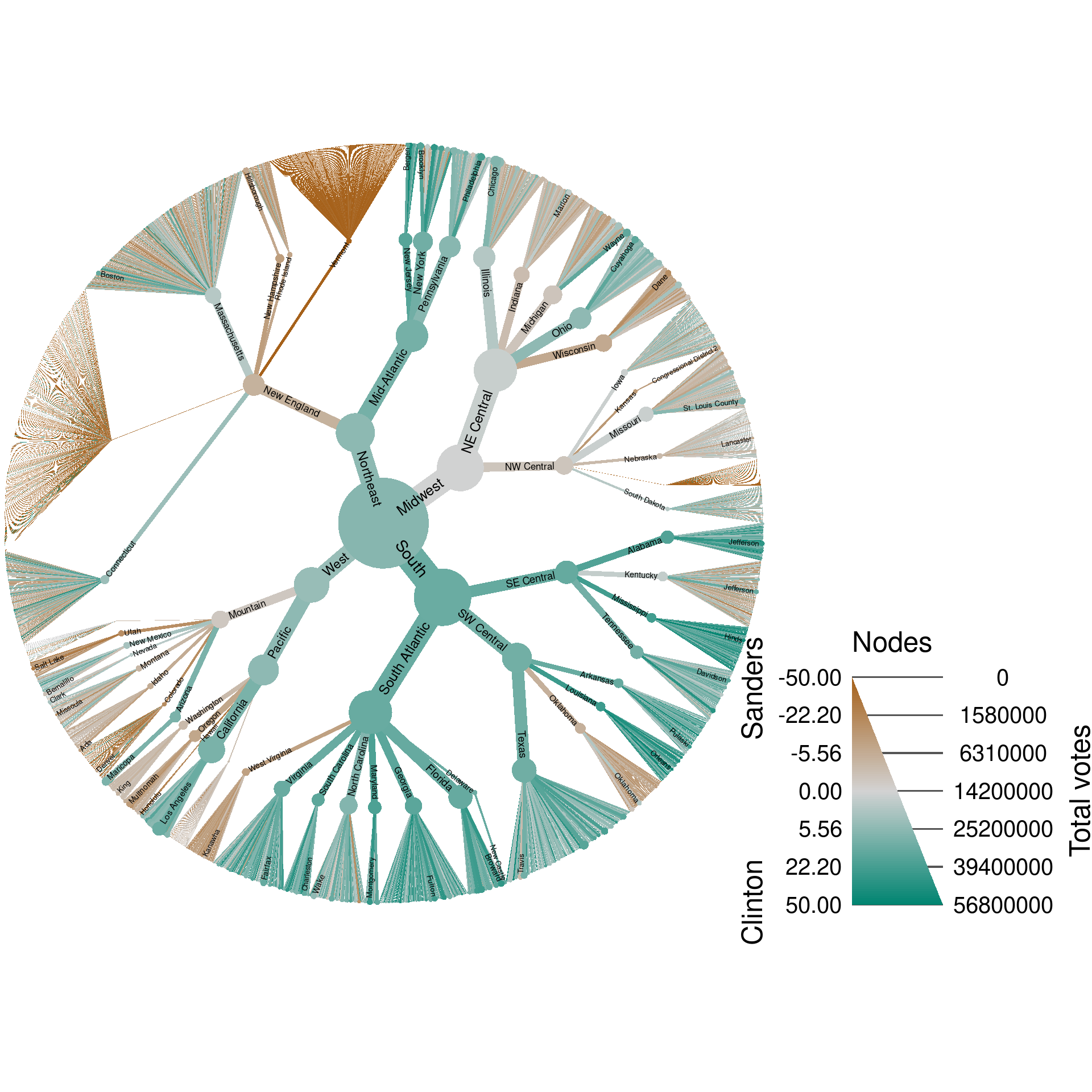
Software and packages used
## R version 4.0.3 (2020-10-10)
## Platform: x86_64-pc-linux-gnu (64-bit)
## Running under: Pop!_OS 20.04 LTS
##
## Matrix products: default
## BLAS:   /usr/lib/x86_64-linux-gnu/blas/libblas.so.3.9.0
## LAPACK: /usr/lib/x86_64-linux-gnu/lapack/liblapack.so.3.9.0
##
## locale:
##  [1] LC_CTYPE=en_US.UTF-8       LC_NUMERIC=C               LC_TIME=en_US.UTF-8
##  [4] LC_COLLATE=en_US.UTF-8     LC_MONETARY=en_US.UTF-8    LC_MESSAGES=en_US.UTF-8
##  [7] LC_PAPER=en_US.UTF-8       LC_NAME=C                  LC_ADDRESS=C
## [10] LC_TELEPHONE=C             LC_MEASUREMENT=en_US.UTF-8 LC_IDENTIFICATION=C
##
## attached base packages:
## [1] stats     graphics  grDevices utils     datasets  methods   base
##
## other attached packages:
## [1] readr_1.4.0          metacoder_0.3.5      stringr_1.4.0        glossary_0.1.0
## [5] knitcitations_1.0.12 knitr_1.30
##
## loaded via a namespace (and not attached):
##  [1] Rcpp_1.0.5        compiler_4.0.3    pillar_1.4.6      plyr_1.8.6        tools_4.0.3
##  [6] ggfittext_0.9.0   digest_0.6.27     gtable_0.3.0      lubridate_1.7.9   jsonlite_1.7.1
## [11] evaluate_0.14     lifecycle_0.2.0   tibble_3.0.4      pkgconfig_2.0.3   rlang_0.4.10
## [16] igraph_1.2.6      bibtex_0.4.2.3    cli_2.1.0         rstudioapi_0.11   yaml_2.2.1
## [21] xfun_0.19         RefManageR_1.2.12 dplyr_1.0.2       httr_1.4.2        xml2_1.3.2
## [26] generics_0.1.0    vctrs_0.3.4       hms_0.5.3         grid_4.0.3        tidyselect_1.1.0
## [31] glue_1.4.2        R6_2.5.0          fansi_0.4.1       rmarkdown_2.5     farver_2.0.3
## [36] ggplot2_3.3.2     purrr_0.3.4       magrittr_2.0.1    scales_1.1.1      htmltools_0.5.1.1
## [41] ellipsis_0.3.1    assertthat_0.2.1  colorspace_1.4-1  labeling_0.4.2    utf8_1.1.4
## [46] stringi_1.5.3     munsell_0.5.0     lazyeval_0.2.2    crayon_1.3.4