
Graphing the Greengenes database
Requirements
NOTE: This analysis requires at least 10Gb of RAM to run. It uses large files not included in the repository and many steps can take a few minutes to run.
Parameters
Analysis input/output
input_folder <- "raw_input" # Where all the large input files are. Ignored by git.
output_folder <- "results" # Where plots will be saved
output_format <- "pdf" # The file format of saved plots
pub_fig_folder <- "publication"
revision_n <- 1
result_path <- function(name) {
  file.path(output_folder, paste0(name, ".", output_format))
}
save_publication_fig <- function(name, figure_number) {
  file.path(result_path(name), paste0("revision_", revision_n), paste0("figure_", figure_number, "--", name, ".", output_format))
}
Analysis parameters
These settings are shared between the RDP, SILVA, and Greengenes analyses, since the results of those three analyeses are combined in one plot later. This ensures that all of the graphs use the same color and size scales, instead of optimizing them for each data set, as would be done automatically otherwise.
size_range <- c(0.0004, 0.015) # The size range of nodes
label_size_range <- c(0.002, 0.05) # The size range of labels
all_size_interval <- c(1, 3000000) # The range of read counts to display in the whole database plots
pcr_size_interval <- c(1, 25000) # The range of read counts to display in the PCR plots
label_max <- 50 # The maximum number of labels to show on each graph
max_taxonomy_depth <- 4 # The maximum number of taxonomic ranks to show
min_seq_count <- NULL # The minimum number of sequeces need to show a taxon.
just_bacteria <- TRUE # If TRUE, only show bacterial taxa
max_mismatch <- 10 # Percentage mismatch tolerated in pcr
pcr_success_cutoff <- 0.90 # Any taxon with a greater proportion of PCR sucess will be excluded from the PCR plots
min_seq_length <- 1200 # Use to encourage full length sequences
forward_primer = c("515F" = "GTGYCAGCMGCCGCGGTAA")
reverse_primer = c("806R" = "GGACTACNVGGGTWTCTAAT")
pcr_success_color_scale = c(viridis::plasma(10)[4:9], "lightgrey")
Parse database
The greengenes database stores sequences in one file and taxonomy information in another and the order of the two files differ making parseing more difficult than the other databases. Since taxonomy inforamtion is needed for creating the taxmap data structure, we will parse it first and add the sequence information on after. The input files are not included in this repository because they are large, but you can download them from the Greengenes website here:
http://greengenes.lbl.gov/Download/
Parse taxonomy file
gg_taxonomy_path <- file.path(input_folder, "gg_13_5_taxonomy.txt")
gg_taxonomy <- readLines(gg_taxonomy_path)
print(gg_taxonomy[1:5])
## [1] "228054\tk__Bacteria; p__Cyanobacteria; c__Synechococcophycideae; o__Synechococcales; f__Synechococcaceae; g__Synechococcus; s__"
## [2] "844608\tk__Bacteria; p__Cyanobacteria; c__Synechococcophycideae; o__Synechococcales; f__Synechococcaceae; g__Synechococcus; s__"
## [3] "178780\tk__Bacteria; p__Cyanobacteria; c__Synechococcophycideae; o__Synechococcales; f__Synechococcaceae; g__Synechococcus; s__"
## [4] "198479\tk__Bacteria; p__Cyanobacteria; c__Synechococcophycideae; o__Synechococcales; f__Synechococcaceae; g__Synechococcus; s__"
## [5] "187280\tk__Bacteria; p__Cyanobacteria; c__Synechococcophycideae; o__Synechococcales; f__Synechococcaceae; g__Synechococcus; s__"
Note that there are some ranks with no names. These will be removed after parsing the file since they provide no information and an uniform-length taxonomy is not needed.
# Parse taxonomy file
greengenes <- extract_tax_data(gg_taxonomy,
                               key = c(id = "info", "class"),
                               regex = "^([0-9]+)\t(.*)$",
                               class_sep = "; ",
                               class_regex = "^([a-z]{1})__(.*)$",
                               class_key = c(rank = "taxon_rank", "taxon_name"))
greengenes$data$class_data <- NULL

# Remove data for ranks with no information
greengenes <- filter_taxa(greengenes, taxon_names != "")
print(greengenes)
## <Taxmap>
## 3093 taxa: aab. Bacteria, aac. Archaea ... kxj. globerulus, kxs. dorotheae
## 3093 edges: NA->aab, NA->aac, aab->aad, aab->aae ... dgr->kxb, eeu->kxj, fco->kxs
## 1 data sets:
## tax_data:
## # A tibble: 1,262,986 x 3
## taxon_id id input
## <chr> <chr> <chr>
## 1 dgl 228054 "228054\tk__Bacteria; p__Cyanobacteria; c__Synechococcophycideae;…
## 2 dgl 844608 "844608\tk__Bacteria; p__Cyanobacteria; c__Synechococcophycideae;…
## 3 dgl 178780 "178780\tk__Bacteria; p__Cyanobacteria; c__Synechococcophycideae;…
## # … with 1,262,983 more rows
## 0 functions:
Parse sequence file
Next we will parse the sequence file so we can add it to the obs_data table of the greengenes object.
gg_sequence_path <- file.path(input_folder, "gg_13_5.fasta")
substr(readLines(gg_sequence_path, n = 10), 1, 100)
## [1] ">1111886"
## [2] "AACGAACGCTGGCGGCATGCCTAACACATGCAAGTCGAACGAGACCTTCGGGTCTAGTGGCGCACGGGTGCGTAACGCGTGGGAATCTGCCCTTGGGTAC"
## [3] ">1111885"
## [4] "AGAGTTTGATCCTGGCTCAGAATGAACGCTGGCGGCGTGCCTAACACATGCAAGTCGTACGAGAAATCCCGAGCTTGCTTGGGAAAGTAAAGTGGCGCAC"
## [5] ">1111883"
## [6] "GCTGGCGGCGTGCCTAACACATGTAAGTCGAACGGGACTGGGGGCAACTCCAGTTCAGTGGCAGACGGGTGCGTAACACGTGAGCAACTTGTCCGACGGC"
## [7] ">1111882"
## [8] "AGAGTTTGATCATGGCTCAGGATGAACGCTAGCGGCAGGCCTAACACATGCAAGTCGAGGGGTAGAGGCTTTCGGGCCTTGAGACCGGCGCACGGGTGCG"
## [9] ">1111879"
## [10] "CCTAATGCATGCAAGTCGAACGCAGCAGGCGTGCCTGGCTGCGTGGCGAACGGCTGACGAACACGTGGGTGACCTGCCCCGGAGTGGGGGATACCCCGTC"
Integrating sequence and taxonomy
We will need to use the Greengenes ID to match up which sequence goes with which row since they are in different orders.
greengenes <- mutate_obs(greengenes, "sequence",
                         setNames(gg_seq[id], greengenes$data$tax_data$taxon_id))
## Adding a new "DNAbin" vector of length 1262986.Subset
Next I will subset the taxa in the dataset (depending on parameter settings). This can help make the graphs less cluttered and make it easier to compare databases.
if (! is.null(min_seq_count)) {
  greengenes <- filter_taxa(greengenes, n_obs >= min_seq_count)
}
if (just_bacteria) {
  greengenes <- filter_taxa(greengenes, taxon_names == "Bacteria", subtaxa = TRUE)
}
if (! is.null(max_taxonomy_depth)) {
  greengenes <- filter_taxa(greengenes, n_supertaxa <= max_taxonomy_depth)
}
print(greengenes)
## <Taxmap>
## 1138 taxa: aab. Bacteria, aad. Cyanobacteria ... dga. [Chloroherpetaceae]
## 1138 edges: NA->aab, aab->aad, aab->aae, aab->aaf ... awi->dfp, bpb->dfq, bfb->dga
## 2 data sets:
## tax_data:
## # A tibble: 1,242,330 x 3
## taxon_id id input
## <chr> <chr> <chr>
## 1 bpm 228054 "228054\tk__Bacteria; p__Cyanobacteria; c__Synechococcophycideae;…
## 2 bpm 844608 "844608\tk__Bacteria; p__Cyanobacteria; c__Synechococcophycideae;…
## 3 bpm 178780 "178780\tk__Bacteria; p__Cyanobacteria; c__Synechococcophycideae;…
## # … with 1,242,327 more rows
## sequence:
## 1242330 DNA sequences in binary format stored in a list.
##
## Mean sequence length: 1401.569
## Shortest sequence: 1111
## Longest sequence: 2368
##
## Labels:
## bpm
## bpm
## bpm
## bpm
## bpm
## bpm
## ...
##
## More than 10 million bases: not printing base composition.
## (Total: 1.74 Gb)
## 0 functions:
Remove chloroplast sequences
These are not bacterial and will bias the in silico PCR results. Note that the invert option makes it so taxa are included that did not pass the filter. This is different than simply using name != "Chloroplast", subtaxa = TRUE since the effects of invert are applied after those of subtaxa.
greengenes <- filter_taxa(greengenes, taxon_names == "Chloroplast", subtaxa = TRUE, invert = TRUE)
print(greengenes)
## <Taxmap>
## 1121 taxa: aab. Bacteria, aad. Cyanobacteria ... dfq. SHAS460, dga. [Chloroherpetaceae]
## 1121 edges: NA->aab, aab->aad, aab->aae, aab->aaf ... awi->dfp, bpb->dfq, bfb->dga
## 2 data sets:
## tax_data:
## # A tibble: 1,242,330 x 3
## taxon_id id input
## <chr> <chr> <chr>
## 1 bpm 228054 "228054\tk__Bacteria; p__Cyanobacteria; c__Synechococcophycideae;…
## 2 bpm 844608 "844608\tk__Bacteria; p__Cyanobacteria; c__Synechococcophycideae;…
## 3 bpm 178780 "178780\tk__Bacteria; p__Cyanobacteria; c__Synechococcophycideae;…
## # … with 1,242,327 more rows
## sequence:
## 1242330 DNA sequences in binary format stored in a list.
##
## Mean sequence length: 1401.569
## Shortest sequence: 1111
## Longest sequence: 2368
##
## Labels:
## bpm
## bpm
## bpm
## bpm
## bpm
## bpm
## ...
##
## More than 10 million bases: not printing base composition.
## (Total: 1.74 Gb)
## 0 functions:
Plot whole database
Although graphing everything can be a bit overwhelming (1121 taxa), it gives an intuitive feel for the complexity of the database:
greengenes_plot_all <- heat_tree(greengenes,
                                 node_size = n_obs,
                                 node_color = n_obs,
                                 node_size_range = size_range * 2,
                                 edge_size_range = size_range,
                                 node_size_interval = all_size_interval,
                                 edge_size_interval = all_size_interval,
                                 node_color_interval = all_size_interval,
                                 edge_color_interval = all_size_interval,
                                 node_label = taxon_names,
                                 node_label_max = label_max,
                                 node_label_size_range = label_size_range,
                                 node_color_axis_label = "Sequence count",
                                 output_file = result_path("greengenes--all"))
print(greengenes_plot_all)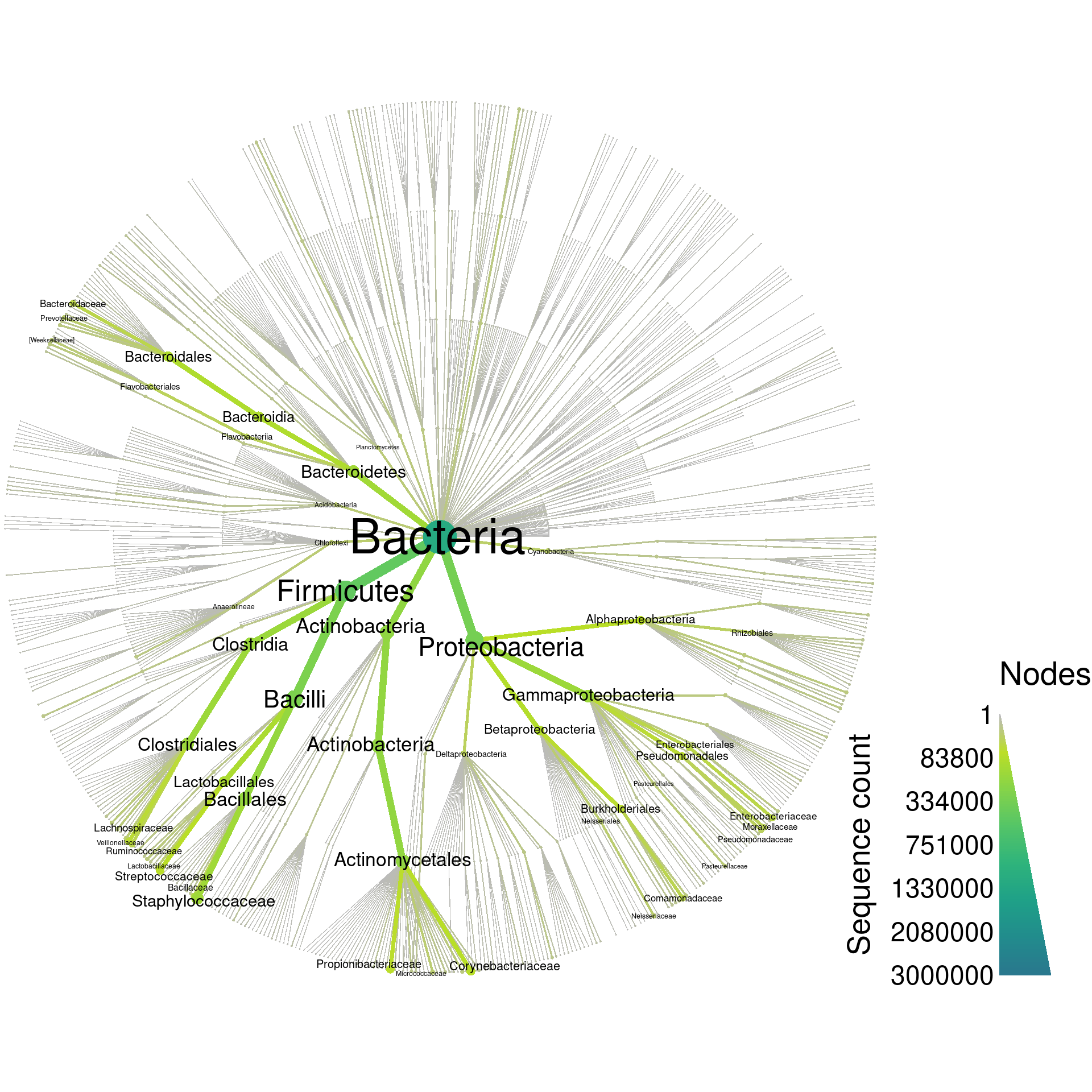
PCR
Before doing the digital PCR, I will filter for only full length sequences, since shorter sequences might not have a primer binding site and the digital PCR would fail, not because of an inability of a real primer to bind to real DNA, but because of missing sequence information in the database. Ideally, this kind of filtering for full length sequences would involve something like a multiple sequences alignment so we don’t remove sequences that are actually full length, but just happen to be shorter than the cutoff of 1200 naturally. However, this method is easy and should work OK.
if (! is.null(min_seq_length)) {
  greengenes <- filter_obs(greengenes, data = c("tax_data", "sequence"), drop_taxa = TRUE,
                           vapply(sequence, length, numeric(1)) >= min_seq_length)
}
print(greengenes)
## <Taxmap>
## 1121 taxa: aab. Bacteria, aad. Cyanobacteria ... dfq. SHAS460, dga. [Chloroherpetaceae]
## 1121 edges: NA->aab, aab->aad, aab->aae, aab->aaf ... awi->dfp, bpb->dfq, bfb->dga
## 2 data sets:
## tax_data:
## # A tibble: 1,242,315 x 3
## taxon_id id input
## <chr> <chr> <chr>
## 1 bpm 228054 "228054\tk__Bacteria; p__Cyanobacteria; c__Synechococcophycideae;…
## 2 bpm 844608 "844608\tk__Bacteria; p__Cyanobacteria; c__Synechococcophycideae;…
## 3 bpm 178780 "178780\tk__Bacteria; p__Cyanobacteria; c__Synechococcophycideae;…
## # … with 1,242,312 more rows
## sequence:
## 1242315 DNA sequences in binary format stored in a list.
##
## Mean sequence length: 1401.572
## Shortest sequence: 1205
## Longest sequence: 2368
##
## Labels:
## bpm
## bpm
## bpm
## bpm
## bpm
## bpm
## ...
##
## More than 10 million bases: not printing base composition.
## (Total: 1.74 Gb)
## 0 functions:
Next I will conduct digital PCR with a new set of universal 16S primers (Walters et al. 2016), allowing for a maximum mismatch of 10%.
greengenes_pcr <- primersearch(greengenes, sequence,
                               forward = forward_primer,
                               reverse = reverse_primer,
                               mismatch = max_mismatch)
Now the object greengenes_pcr has all the information that greengenes has plus the results of the digital PCR. Lets plot the whole database again, but coloring based on digital PCR success.
greengenes_plot_pcr_all <- heat_tree(greengenes_pcr,
                                     node_size = seq_count,
                                     node_size_range = size_range * 2,
                                     edge_size_range = size_range,
                                     node_size_interval = all_size_interval,
                                     edge_size_interval = all_size_interval,
                                     node_label = taxon_names,
                                     node_color = prop_amplified,
                                     node_color_range =  pcr_success_color_scale,
                                     node_color_trans = "linear",
                                     node_label_max = label_max,
                                     node_label_size_range = label_size_range,
                                     edge_color_interval = c(0, 1),
                                     node_color_interval = c(0, 1),
                                     node_color_axis_label = "Proportion PCR success",
                                     node_size_axis_label = "Sequence count",
                                     output_file = result_path("greengenes--pcr_all"))
print(greengenes_plot_pcr_all)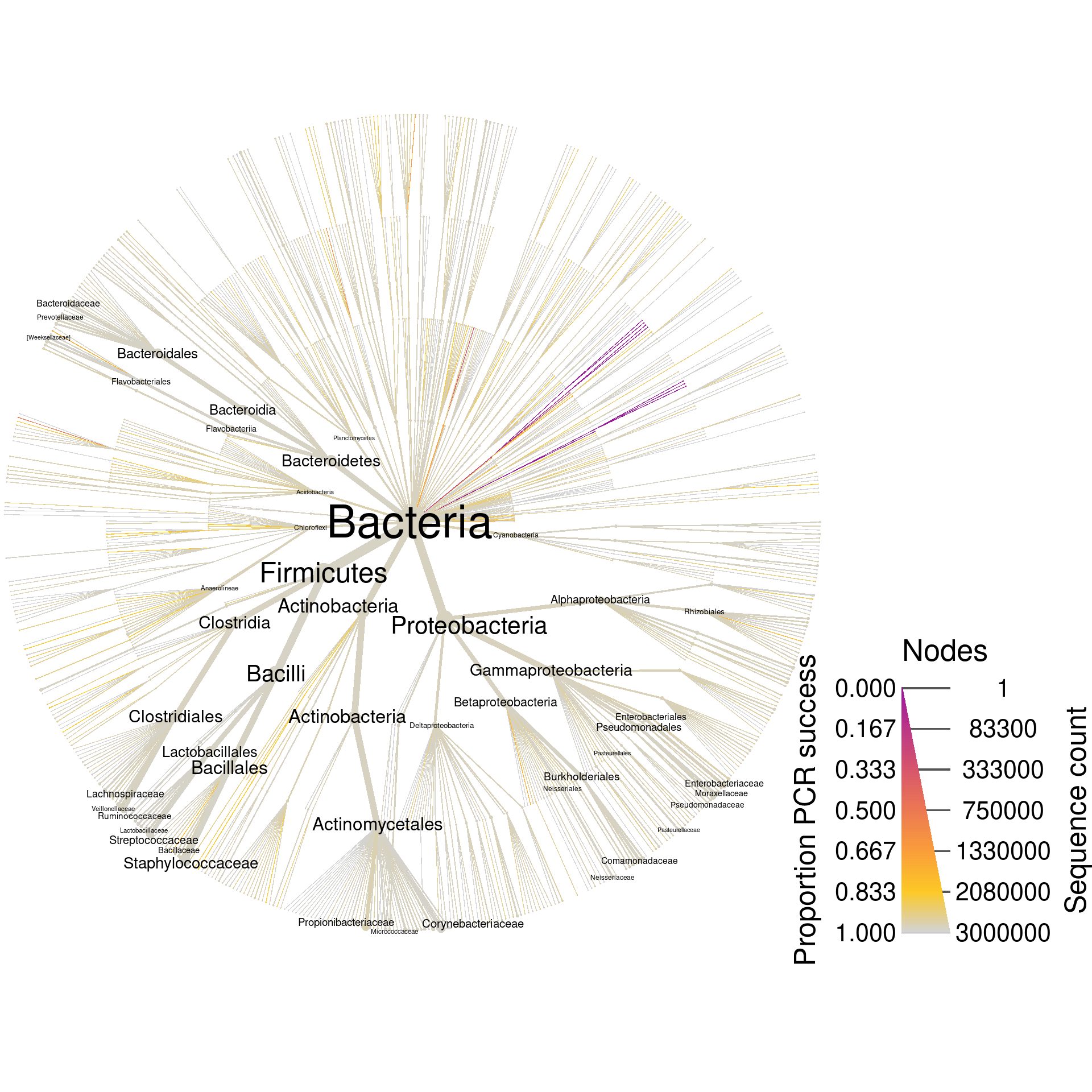
Since these are universal bacterial primers, we would expect most of the database to amplify. The plot shows this and very few sequences were not amplified. If we wanted to look at only those sequences that did not amplify, we could filter taxa by PCR success and plot what remains. I am including the supertaxa of those taxa that did not amplify since excluding them would split the tree into a cloud of fragments lacking taxonomic context.
greengenes_plot_pcr_fail <- greengenes_pcr %>%
  filter_taxa(prop_amplified < pcr_success_cutoff, supertaxa = TRUE) %>%
  heat_tree(node_size = query_count - seq_count,
            node_label = taxon_names,
            node_color = prop_amplified,
            node_size_range = size_range * 2,
            edge_size_range = size_range,
            node_size_interval = pcr_size_interval,
            edge_size_interval = pcr_size_interval,
            node_color_range =  pcr_success_color_scale,
            node_color_trans = "linear",
            node_color_interval = c(0, 1),
            edge_color_interval = c(0, 1),
            node_label_size_range = label_size_range,
            node_label_max = label_max,
            node_color_axis_label = "Proportion PCR success",
            node_size_axis_label = "Sequences not amplified",
            output_file = result_path("greengenes--pcr_fail"))
print(greengenes_plot_pcr_fail)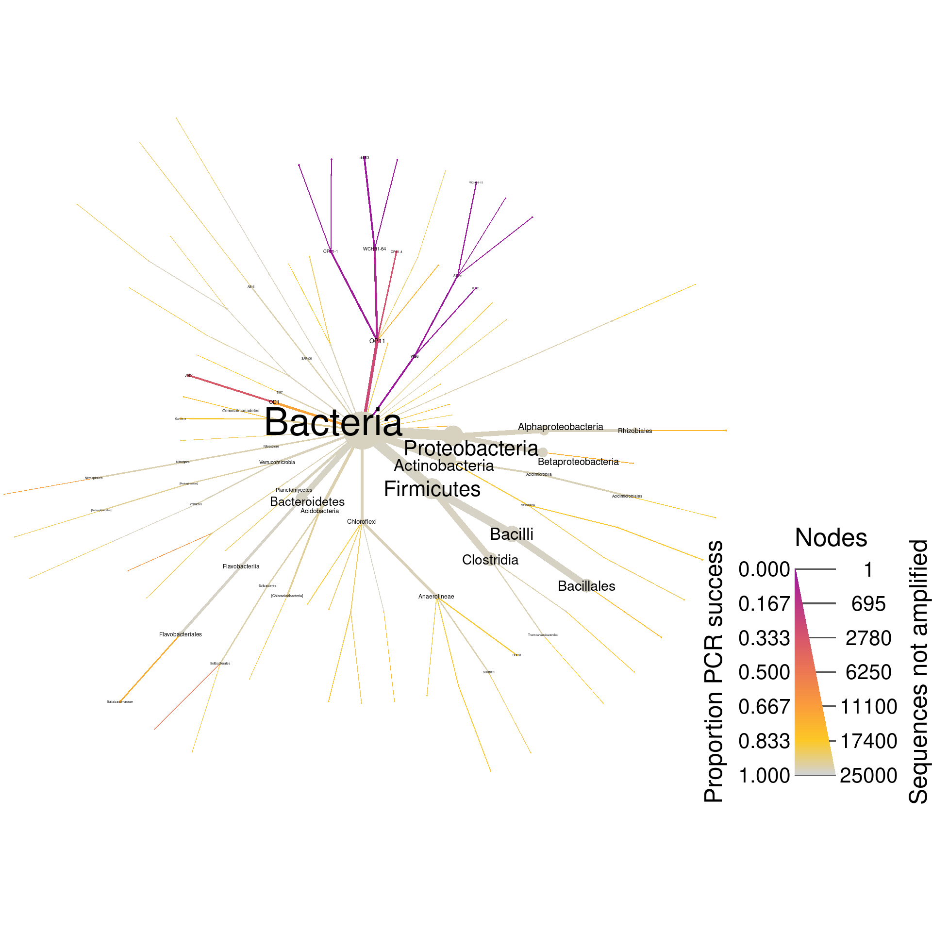
Save outputs for composite figure
Some results from this file will be combined with others from similar analyses to make a composite figure. Below, the needed objects are saved so that they can be loaded by another Rmd file.
Software and packages used
## R version 4.0.3 (2020-10-10)
## Platform: x86_64-pc-linux-gnu (64-bit)
## Running under: Pop!_OS 20.04 LTS
##
## Matrix products: default
## BLAS:   /usr/lib/x86_64-linux-gnu/blas/libblas.so.3.9.0
## LAPACK: /usr/lib/x86_64-linux-gnu/lapack/liblapack.so.3.9.0
##
## locale:
##  [1] LC_CTYPE=en_US.UTF-8       LC_NUMERIC=C               LC_TIME=en_US.UTF-8
##  [4] LC_COLLATE=en_US.UTF-8     LC_MONETARY=en_US.UTF-8    LC_MESSAGES=en_US.UTF-8
##  [7] LC_PAPER=en_US.UTF-8       LC_NAME=C                  LC_ADDRESS=C
## [10] LC_TELEPHONE=C             LC_MEASUREMENT=en_US.UTF-8 LC_IDENTIFICATION=C
##
## attached base packages:
## [1] stats     graphics  grDevices utils     datasets  methods   base
##
## other attached packages:
## [1] metacoder_0.3.5      stringr_1.4.0        glossary_0.1.0       knitcitations_1.0.12
## [5] knitr_1.30
##
## loaded via a namespace (and not attached):
##  [1] progress_1.2.2    tidyselect_1.1.0  xfun_0.19         purrr_0.3.4       lattice_0.20-41
##  [6] colorspace_1.4-1  vctrs_0.3.4       generics_0.1.0    htmltools_0.5.1.1 viridisLite_0.3.0
## [11] yaml_2.2.1        utf8_1.1.4        rlang_0.4.10      pillar_1.4.6      glue_1.4.2
## [16] lifecycle_0.2.0   plyr_1.8.6        ggfittext_0.9.0   munsell_0.5.0     gtable_0.3.0
## [21] codetools_0.2-16  evaluate_0.14     labeling_0.4.2    parallel_4.0.3    fansi_0.4.1
## [26] Rcpp_1.0.5        readr_1.4.0       scales_1.1.1      jsonlite_1.7.1    farver_2.0.3
## [31] gridExtra_2.3     ggplot2_3.3.2     hms_0.5.3         digest_0.6.27     stringi_1.5.3
## [36] dplyr_1.0.2       ade4_1.7-16       grid_4.0.3        bibtex_0.4.2.3    cli_2.1.0
## [41] tools_4.0.3       magrittr_2.0.1    lazyeval_0.2.2    tibble_3.0.4      RefManageR_1.2.12
## [46] crayon_1.3.4      ape_5.4-1         seqinr_4.2-4      pkgconfig_2.0.3   MASS_7.3-53
## [51] ellipsis_0.3.1    prettyunits_1.1.1 xml2_1.3.2        lubridate_1.7.9   assertthat_0.2.1
## [56] rmarkdown_2.5     httr_1.4.2        viridis_0.5.1     R6_2.5.0          igraph_1.2.6
## [61] nlme_3.1-149      compiler_4.0.3
References
Walters, William, Embriette R Hyde, Donna Berg-Lyons, Gail Ackermann, Greg Humphrey, Alma Parada, Jack A Gilbert, et al. 2016. “Improved Bacterial 16S rRNA Gene (V4 and V4-5) and Fungal Internal Transcribed Spacer Marker Gene Primers for Microbial Community Surveys.” mSystems 1 (1): e00009–15.