Getting Started

Before You Start

In the following example, we demonstrate key package functionality using the test data set that is included in the package
You can follow along because all test data and associated CSV input files are contained in the package.
Additional examples are also available under Example Vignettes

Components of the test dataset

Paired-end short read amplicon data

Files: S1_R1.fastq.gz, S1_R2.fastq.gz, S2_R1.fastq.gz, S2_R1.fastq.gz
The files must be zipped and end in either R1.fastq.gz or R2.fastq.gz and each sample must have both R1 and R2 files.

metadata.csv

New row for each unique sample
Samples entered twice if samples contain two pooled metabarcodes, as in the test data template

primerinfo_params.csv

New row for each unique barcode and associated primer sequence
Optional Cutadapt and DADA2 parameters

Taxonomy databases

UNITE fungal database (abridged version)
oomyceteDB

Format of the paired-end read files

The package takes forward and reverse Illumina short read sequence data.
Format of file names To avoid errors, the only characters that are acceptable in sample names are letters and numbers. Characters can be separated by underscores, but no other symbols. The files must end with the suffix R1.fastq.gz or R2.fastq.gz.

Format of metadata file

The format of the CSV file named metadata.csv is simple.
A template is here.
The only two required columns (with these headers) are:
- Column 1. sample_name
- Column 2. primer_info (applicable options: ‘rps10’, ‘its’, ‘r16S’, ‘other1’, other2’)

Additional columns

Other columns should be pasted after these two columns.
They can be referenced later during the analysis steps and save a step of loading metadata later.

Notes

S1 and S2 are come from a rhododendron rhizobiome dataset and are a random subset of the full set of reads.
S1 and S2 are included twice in the ‘metadata.csv’ sheet. This is because these two samples contain pooled metabarcodes (ITS1 and rps10).
To demultiplex and run both analyses in tandem, include the same sample twice under sample_name, and then change the primer_name.

Here is what the metadata.csv looks like for this test dataset:

sample_name	primer_name	organism
S1	rps10	Cry
S2	rps10	Cin
S1	its	Cry
S2	its	Cin

Format of primer and parameters file

Primer sequence information and user-defined parameters are placed in primerinfo_params.csv

To simplify how functions are called, user will provide parameters within this input file.
We recommend using the template linked here.
Remember to add any additional optional DADA2 parameters you want to use.
The only three required columns (with these headers) are:
- Column 1. sample_name
- Column 2. forward (primer sequence)
- Column 3. reverse(primer sequence)

Example template for primerinfo_params.csv

primer_name	forward	reverse	already_trimmed	minCutadaptlength	multithread	verbose	maxN	maxEE_forward	maxEE_reverse	truncLen_forward	truncLen_reverse	truncQ	minLen	maxLen	minQ	trimLeft	trimRight	rm.lowcomplex	minOverlap	maxMismatch	min_asv_length
rps10	GTTGGTTAGAGYARAAGACT	ATRYYTAGAAAGAYTYGAACT	FALSE	100	TRUE	FALSE	1.00E+05	5	5	0	0	5	150	Inf	0	0	0	0	15	0	50
its	CTTGGTCATTTAGAGGAAGTAA	GCTGCGTTCTTCATCGATGC	FALSE	50	TRUE	FALSE	1.00E+05	5	5	0	0	5	50	Inf	0	0	0	0	15	0	50

For more info on parameter specifics, see Documentation

Reference Database Format

For now, the package is compatible with the following databases:
- oomycetedb from: https://grunwaldlab.github.io/OomyceteDB/
- SILVA 16S database with species assignments: https://www.arb-silva.de/
- UNITE fungal database from https://unite.ut.ee/repository.php
- A user can select up to two other databases, but will first need to reformat headers exactly like the SILVA database headers.
  - See more in the ‘Documentation’ tab.

Databases are downloaded from these sources and then placed in the from the user-specified data folder where raw data files and csv files are located.

Additional Notes

Computer specifications may be a limiting factor.
If you are using the SILVA or UNITE databases for taxonomic assignment steps, an ordinary personal computer (unless it has sufficient RAM) may not have enough memory for the taxonomic assignment steps, even with few samples.
The test databases and reads are subsetted and the following example should run on a personal computer with at least 16 GB of RAM.
If computer crashes during the taxonomic assignment step, you will need to switch to a computer with sufficient memory.
You must ensure that you have enough storage to save intermediate files in a temporary directory (default) or user-specified directory before proceeding.

Installation

Dependencies:
First install Cutadapt program following the instructions here: https://cutadapt.readthedocs.io/en/stable/installation.html

Let’s locate where the Cutadapt executable is.

You must do this from a Terminal window:

#If you installed with pip or pipx, or homebrew, run this command from a Terminal window
which cutadapt
cutadapt --version

If you followed the cutadapt installation instructions to create a conda environment called Cutadapt (change to whatever you named your environment), to install it in.

Open up a Terminal window and type these commands:

#Run commands from a Terminal window
conda activate cutadapt
which cutadapt
cutadapt --version

Second, make sure the following R packages are installed:

DADA2 (Latest version is 3.20)
- To install, follow these instructions: https://www.bioconductor.org/packages/release/bioc/html/dada2.html
phyloseq
- To install: https://www.bioconductor.org/packages/release/bioc/html/phyloseq.html
metacoder (Available through CRAN)

To install the development version of package (while submission to CRAN is in progress):

Loading the Package

For now, the package will be loaded by retrieving it from GitHub. Submission to CRAN is in progress.

#Here we install demulticoder (instructions will be updated once available through CRAN)
devtools::install_github("grunwaldlab/demulticoder")
library("demulticoder")
#Let's make sure other packages are loaded:
library("devtools")
library("dada2")
library("phyloseq")
library("metacoder")

Reorganize data tables and set-up data directory structure

The sample names, primer sequences, and other metadata are reorganized in preparation for running Cutadapt to remove primers.

output<-prepare_reads(
  data_directory = system.file("extdata", package = "demulticoder"),
  output_directory = tempdir(), # Change to your desired output directory path or leave as is", 
  overwrite_existing = TRUE)
#> Existing files found in the output directory. Overwriting existing files.
#> Rows: 2 Columns: 25
#> ── Column specification ────────────────────────────────────────────────────────
#> Delimiter: ","
#> chr  (3): primer_name, forward, reverse
#> dbl (18): minCutadaptlength, maxN, maxEE_forward, maxEE_reverse, truncLen_fo...
#> lgl  (4): already_trimmed, count_all_samples, multithread, verbose
#> 
#> ℹ Use `spec()` to retrieve the full column specification for this data.
#> ℹ Specify the column types or set `show_col_types = FALSE` to quiet this message.
#> Rows: 2 Columns: 25
#> ── Column specification ────────────────────────────────────────────────────────
#> Delimiter: ","
#> chr  (3): primer_name, forward, reverse
#> dbl (18): minCutadaptlength, maxN, maxEE_forward, maxEE_reverse, truncLen_fo...
#> lgl  (4): already_trimmed, count_all_samples, multithread, verbose
#> 
#> ℹ Use `spec()` to retrieve the full column specification for this data.
#> ℹ Specify the column types or set `show_col_types = FALSE` to quiet this message.
#> Rows: 4 Columns: 3
#> ── Column specification ────────────────────────────────────────────────────────
#> Delimiter: ","
#> chr (3): sample_name, primer_name, organism
#> 
#> ℹ Use `spec()` to retrieve the full column specification for this data.
#> ℹ Specify the column types or set `show_col_types = FALSE` to quiet this message.
#> Creating output directory: /tmp/RtmpWjJW7o/demulticoder_run/prefiltered_sequences

Remove primers with Cutadapt

Before running Cutadapt, please ensure that you have installed it

cut_trim(
  output,
  cutadapt_path = "/usr/bin/cutadapt", #CHANGE LOCATION TO YOUR LOCAL INSTALLATION
  overwrite_existing = TRUE)
#> Running cutadapt 3.5 for its sequence data

#> Running cutadapt 3.5 for rps10 sequence data

ASV inference step

Raw reads will be merged and ASVs will be inferred

make_asv_abund_matrix(
  output,
  overwrite_existing = TRUE)
#> 80608 total bases in 307 reads from 2 samples will be used for learning the error rates.
#> Sample 1 - 163 reads in 84 unique sequences.
#> Sample 2 - 144 reads in 96 unique sequences.
#> 82114 total bases in 307 reads from 2 samples will be used for learning the error rates.
#> Sample 1 - 163 reads in 128 unique sequences.
#> Sample 2 - 144 reads in 119 unique sequences.

#> 91897 total bases in 327 reads from 2 samples will be used for learning the error rates.
#> Sample 1 - 145 reads in 107 unique sequences.
#> Sample 2 - 182 reads in 133 unique sequences.
#> 91567 total bases in 327 reads from 2 samples will be used for learning the error rates.
#> Sample 1 - 145 reads in 114 unique sequences.
#> Sample 2 - 182 reads in 170 unique sequences.

#> $its
#> [1] "/tmp/RtmpWjJW7o/demulticoder_run/asvabund_matrixDADA2_its.RData"
#> 
#> $rps10
#> [1] "/tmp/RtmpWjJW7o/demulticoder_run/asvabund_matrixDADA2_rps10.RData"

Taxonomic assignment step

Using the core assignTaxonomy function from DADA2, taxonomic assignments will be given to ASVs.

assign_tax(
  output,
  asv_abund_matrix,
  retrieve_files=TRUE,
  overwrite_existing = TRUE)
#>   samplename_barcode input filtered denoisedF denoisedR merged nonchim
#> 1             S1_its   299      163       146       141    132     132
#> 2             S2_its   235      144       113        99     99      99
#>   samplename_barcode input filtered denoisedF denoisedR merged nonchim
#> 1           S1_rps10   196      145       145       145    145     145
#> 2           S2_rps10   253      182       181       181    181     181

Format of output matrices

The default output is a CSV file per metabarcode with the inferred ASVs and sequences, taxonomic assignments, and bootstrap supports provided by DADA2. These data can then be used as input for downstream steps.
To view these files, locate the files with the prefix final_asv_abundance_matrix in your specified output directory.
In this example, it will be in the home directory within demulticoder_test.
You can then open your matrices using Excel
We recommend checking the column with the ASV sequences to make sure there aren’t truncated sequences *It is important to also review the column showing the taxonomic assignments of each ASV and their associated bootstrap supports.

We can also load the matrices into our R environment and view then from R Studio.

We do that here with the rps10 matrix

rps10_matrix<-read.csv("~/demulticoder_test/final_asv_abundance_matrix_rps10.csv", header=TRUE)
head(rps10_matrix)
#>   asv_id
#> 1  asv_1
#> 2  asv_2
#> 3  asv_3
#> 4  asv_4
#> 5  asv_5
#>                                                                                                                                                                                                                                                                                                                                                                                                                                                    sequence
#> 1 GAAAATCTTTGTGTCGGTGGTTCAAATCCACCTCCAGACAAATTAATTTTTTAAAACTTATGTTTATATTAAGAATTACATTTAAATCTATTAAAAAAATAAATAACATTAAACCTATTTTATTAAATCAAAAAAATTTAAATAAATTTAATAATATTAAAATAAATGGAATATTTAAAACAAAAAATAAAAATAAAATTTTTACAGTATTAAAATCACCACATGTTAATAAAAAAGCACGTGAACATTTTATTTATAAAAATTTTACACAAAAAGTTGAAATTAAATGTTTAAATATTTTTCAATTATTAAATTTTTTAATTTTGATTAAAAAAATCTTAACAGAAAATTTTATTATTACTACAAAAATAATTAAACAATAATTAATATATGCTTATAGCTTAATGGATAAAGCATTAGATTGCGGATCTACAAAATGAA
#> 2    GAAAATCTTTGTGTCGGTGGTTCAAGTCCGCCTCCAAACATCTTATAAAAATGTATGTATATTTTACGAATTAGTTTTAAATCAGTAGAAAAAATAAATGAATTAAAAAAAAATATCTCAAAAATAAAAAAAATATATAATTTTAAAAATTTAAAAGTAAATGGTATTTTTAGAACAAAAAATAAAAATAAAATTTTTACATTATTAAAATCACCCCATGTTAATAAAAAATCACGTGAACATTTTATATATAAAAATTATATTCAAAAAATTGATTTAAATTTTTCAAATTTTTTTCAATTATTAAATTTTTTAGTAATTTTAAAAAAAATATTATCTAAAGATTTTTTAATCAATATCAAAATTATTAAAAAAAATAAAAAAAATATGCTTATAGCTTAATGGATAAAGCGTTAGATTGCGGATCTATAAAATGAA
#> 3      GAAAATCTTTGTGTCGGTGGTTCAAGTCCACCTCCAGACAAAAATAATAACTATGTATATTTTAAGAATAACTTTTAAATCAATACAAAAAATAAATAATATTAAAAAAAATTTATTAAAATTAAAAAAAATAAATAAATTTAAAAATATTCAAATAAAAGGAATATTTAAAATAAAAGATAAAAATAAAATTTTTACTTTATTAAAATCACCTCACGTAAATAAAAAATCTCGTGAACATTTTATTTATAAAAATTATACTCAAAAAATAGATGTAAAATTTTCAAATATTATTGAATTATTTAATTTTATAATACTTATTAAAAAAGTTTTAACTAAAAATTTTATAATAAATTTTAAAATTATAAAATATAATAAAAAAAAAATGCTTATAGCTTAATGGATAAAGCGTTAGATTGCGGATCTATAAAATGAA
#> 4  GAAAATCTTTGTGTCGGTGGTTCAAATCCGCCTCCAAACAAAAATATAAATTATTTTATATGTATATTTTAAGAATAAGTTTTAAATCTGTATCAAAAATAGATAAAATTAAAAAAGAATTATCAAGATTAAAAAAAATATATAATTTTAAAAATATAACAATTAATGGTATTTTTAAAACAAAAAATAAAGATAAAATTTTTACATTATTAAAATCACCTCATGTTAATAAAAAATCTCGCGAACATTTTATTTATAAAAATTATGTACAAAAAATAGATTTAAATTTTATTAATATTTTTCAATTAATAAATTTTTTAATAATTTTAAAAAAAAAATTATCAAAAAATGTATTAATAAATGTAAAAATAATTAAAAAATAAAAAAATATGCTTATAGCTTAATGGATAAAGCGTTAGATTGCGGATCTATAAAATGAA
#> 5    GAAAATCTTTGTGTCGGTGGTTCAAGTCCGCCTCCAAACATCTTATAAAAATGTATGTATATTTTACGAATTAGTTTTAAATCAGTAGAAAAAATAAATGAATTAAAAAAAAATATCTCAAAAATAAAAAAAATATATAATTTTAAAAATTTAAAAGTAAAATGGTATTTTTAGAACAAAAAATAAAAATAAAATTTTTACATTATTAAAATCACCCCATGTTAATAAAAAATCACGTGAACATTTTATATATAAAAATTATATTCAAAAAATTGATTTAAATTTTTCAAATTTTTTTCAATTATTAAATTTTTTAGTAATTTTAAAAAAAACATTATCTAAAGATTTTTTAATCAATATTAAAATTATTAAAAAAAATAAAAAAATATGCTTATAGCTTAATGGATAAAGCGTTAGATTGCGGATCTATAAAATGAA
#>                                                                                                                                                                                                                   dada2_tax
#> 1 Stramenopila--100--Kingdom;Oomycota--100--Phylum;Oomycetes--100--Class;Peronosporales--26--Order;Peronosporaceae--26--Family;Phytophthora--23--Genus;Phytophthora_sp.kununurra--13--Species;oomycetedb_650--13--Reference
#> 2                    Stramenopila--100--Kingdom;Oomycota--100--Phylum;Oomycetes--100--Class;Pythiales--100--Order;Pythiaceae--100--Family;Pythium--100--Genus;Pythium_dissotocum--49--Species;oomycetedb_749--24--Reference
#> 3 Stramenopila--100--Kingdom;Oomycota--100--Phylum;Oomycetes--100--Class;Pythiales--100--Order;Pythiaceae--100--Family;Globisporangium--100--Genus;Globisporangium_cylindrosporum--22--Species;oomycetedb_41--22--Reference
#> 4                   Stramenopila--100--Kingdom;Oomycota--100--Phylum;Oomycetes--100--Class;Pythiales--94--Order;Pythiaceae--94--Family;Pythium--89--Genus;Pythium_aphanidermatum--19--Species;oomycetedb_727--19--Reference
#> 5                    Stramenopila--100--Kingdom;Oomycota--100--Phylum;Oomycetes--100--Class;Pythiales--100--Order;Pythiaceae--100--Family;Pythium--100--Genus;Pythium_oopapillum--67--Species;oomycetedb_771--67--Reference
#>   S1_rps10 S2_rps10
#> 1      842       17
#> 2      578      220
#> 3        0      587
#> 4        0      516
#> 5        0      163

We can also inspect the first rows of the ITS1 matrix

its_matrix<-read.csv("~/demulticoder_test/final_asv_abundance_matrix_its.csv", header=TRUE)
head(its_matrix)
#>   asv_id
#> 1  asv_1
#> 2  asv_2
#> 3  asv_3
#> 4  asv_4
#> 5  asv_5
#> 6  asv_6
#>                                                                                                                                                                                                                                                                                                                                 sequence
#> 1                                              AAAAAGTCGTAACAAGGTTTCCGTAGGTGAACCTGCGGAAGGATCATTAGTGAATCTTCAAAGTCGGCTCGTCAGATTGTGCTGGTGGAGACACATGTGCACGTCTACGAGTCGCAAACCCACACACCTGTGCATCTATGACTCTGAGTGCCGCTTTGCATGGCCCCTTGATTTGGGCCTGGCGCTCGAGTACTTTCACACACTCTCGAATGTAATGGAATGTCTTCTTGTGCATAACGTACAAACAGAAACAACTTTCAACAACGGATCTCTTGGCTCTC
#> 2                                              AAAAAGTCGTAACAAGGTTTCCGTAGGTGAACCTGCGGAAGGATCATTAGTGAATCTTCAAAGTCGGCTCGTCGGATTGTGCTGGTGGAGACACATGTGCACGTCTACGAGTCGCAAACCCACACACCTGTGCATCTATGACTCTGAGTGCCGCTTTGCATGGCCCCTTGATTTGGGCCTGGCGCTCGAGTACTTTCACACACTCTCGAATGTAATGGAATGTCTTGTTGTGCATAACGTACAAACAGAAACAACTTTCAACAACGGATCTCTTGGCTCTC
#> 3                                              AAAAAGTCGTAACAAGGTTTCCGTAGGTGAACCTGCGGAAGGATCATTAGTGAATCTTCAAAGTCGGCTCGTCGGATTGTGCTGGTGGAGACACATGTGCACGTCTACGAGTCGCAAACCCACACACCTGTGCATCTATGACTCTGAGTGCCGCTTTGCATGGCCCCTTGATTTGGGCCTGGCGCTCGAGTACTTTCACACACTCTCGAATGTAATGGAATGACTTGTTGTGCATAACGTACAAACAGAAACAACTTTCAACAACGGATCTCTTGGCTCTC
#> 4 AAGTCGTAACAAGGTTTCCGTAGGTGAACCTGCGGAAGGATCATTAACGAGTTCAACTGGGGTCTGTGGGGATTCGATGCTGGCCTCCGGGCATGTGCTCGTCCCCCGGACCTCACATCCACTCACAACCCCTGTGCATCATGAGAGGTGTGGTCCTCCGTCATGGGAGCAGCTCCCCTCCGGGCGTGTTTGTACACCCCGGGCGGTCGAGCCGGGACTGCACTTCGACGCCTTTACACAAACCTTTGAATCAGTGATGTAGAATGTCATGGCCAGCGATGGTCGAACTTTAAATACAACTTTCAACAACGGATCTCTTGGCTCTC
#> 5                                              AAAAAGTCGTAACAAGGTTTCCGTAGGTGAACCTGCGGAAGGATCATTAGTGAATCTTCAAAGTCGGCTCGTCGGATTGTGCTGGTGGAGACACATGTGCACATCTACGAGTCGCAAACCCACACACCTGTGCATCTATGACTCTGAGTGCCGCTTTGCATGGCCCCTTGATTTGGGCCTGGCGCTCGAGTACTTTCACACACTCTCGAATGTAATGGAATGTCTTGTTGTGCATAACGTACAAACAGAAACAACTTTCAACAACGGATCTCTTGGCTCTC
#> 6                                                                                                    AAGTCGTAACAAGGTTTCCGTAGGTGAACCTGCGGAAGGATCATTAAAAATGAAGCCGGGAAACCGGTCCTTCTAACCCTTGATTATCTTAATTTGTTGCTTTGGTGGGCCGCGCAAGCACCGGCTTCGGCTGGATCGTGCCCGCCAGAGGACCACAACTCTGTATCAAATGTCGTCTGAGTACTATATAATAGTTAAAACTTTCAACAACGGATCTCTTGGTTCTG
#>                                                                                                                                                                        dada2_tax
#> 1 Fungi--100--Kingdom;Basidiomycota--100--Phylum;Agaricomycetes--100--Class;Sebacinales--100--Order;unidentified--98--Family;unidentified--98--Genus;Sebacinales_sp--98--Species
#> 2 Fungi--100--Kingdom;Basidiomycota--100--Phylum;Agaricomycetes--100--Class;Sebacinales--100--Order;unidentified--97--Family;unidentified--97--Genus;Sebacinales_sp--97--Species
#> 3 Fungi--100--Kingdom;Basidiomycota--100--Phylum;Agaricomycetes--100--Class;Sebacinales--100--Order;unidentified--99--Family;unidentified--99--Genus;Sebacinales_sp--99--Species
#> 4 Fungi--100--Kingdom;Basidiomycota--62--Phylum;Agaricomycetes--59--Class;Hymenochaetales--21--Order;Repetobasidiaceae--8--Family;Rickenella--8--Genus;Rickenella_sp--8--Species
#> 5 Fungi--100--Kingdom;Basidiomycota--100--Phylum;Agaricomycetes--100--Class;Sebacinales--100--Order;unidentified--96--Family;unidentified--96--Genus;Sebacinales_sp--96--Species
#> 6         Fungi--100--Kingdom;Ascomycota--100--Phylum;Leotiomycetes--98--Class;Helotiales--98--Order;unidentified--86--Family;unidentified--86--Genus;Helotiales_sp--86--Species
#>   S1_its S2_its
#> 1    436      0
#> 2    405      0
#> 3      0    299
#> 4    209     65
#> 5      0    200
#> 6     16    116

Reformat ASV matrix as `taxmap` and `phyloseq` objects after optional filtering of low abundance ASVs

objs<-convert_asv_matrix_to_objs(output, minimum_bootstrap = 0, save_outputs = TRUE)

Objects can now be used for downstream data analysis

Here we make heattrees using taxmap object.

First we make a heat tree to examine fungal community composition using our ITS1 data.

objs$taxmap_its %>%
  filter_taxa(! grepl(x = taxon_names, "NA", ignore.case = TRUE)) %>%
  metacoder::heat_tree(node_label = taxon_names,
                       node_size = n_obs,
                       node_color = n_obs,
                       node_color_axis_label = "ASV count",
                       node_size_axis_label = "Total Abundance of Taxa",
                       layout = "da", initial_layout = "re")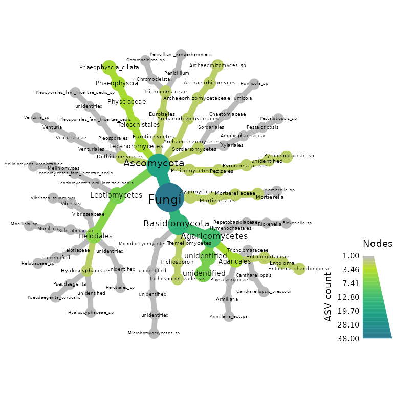

Now we make a heat tree to showcase oomycete community composition using our rps10 data

objs$taxmap_rps10 %>%
  filter_taxa(! grepl(x = taxon_names, "NA", ignore.case = TRUE)) %>%
  metacoder::heat_tree(node_label = taxon_names,
                       node_size = n_obs,
                       node_color = n_obs,
                       node_color_axis_label = "ASV count",
                       node_size_axis_label = "Total Abundance of Taxa",
                       layout = "da", initial_layout = "re")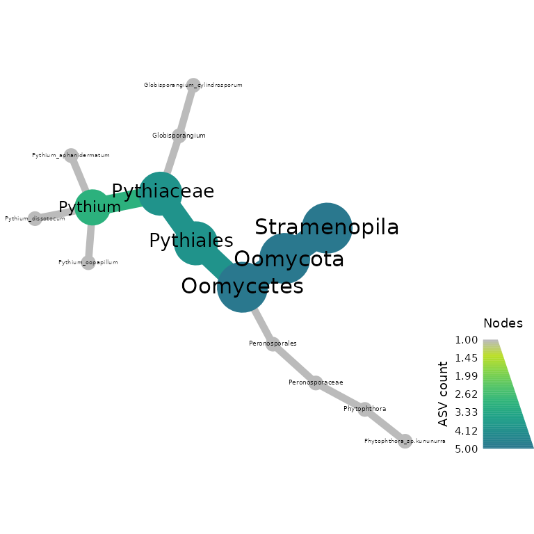

We can also do a variety of analyses, if we convert to phyloseq object

Here we demonstrate how to make a stacked bar plot of the relative abundance of taxa by sample for the ITS1-barcoded samples

data <- objs$phyloseq_its %>%
  phyloseq::transform_sample_counts(function(x) {x/sum(x)} ) %>% 
  phyloseq::psmelt() %>%                                        
  dplyr::filter(Abundance > 0.02) %>%                      
  dplyr::arrange(Genus)                                      

abund_plot <- ggplot2::ggplot(data, ggplot2::aes(x = Sample, y = Abundance, fill = Genus)) + 
  ggplot2::geom_bar(stat = "identity", position = "stack", color = "black", size = 0.2) +
  ggplot2::scale_fill_viridis_d() +
  ggplot2::theme_minimal() +
  ggplot2::labs(
    y = "Relative Abundance",
    title = "Relative abundance of taxa by sample",
    fill = "Genus"
  ) +
  ggplot2::theme(
    axis.text.x = ggplot2::element_text(angle = 90, hjust = 1, vjust = 0.5, size = 14),
    panel.grid.major = ggplot2::element_blank(),
    panel.grid.minor = ggplot2::element_blank(),
    legend.position = "top",
    legend.text = ggplot2::element_text(size = 14),
    legend.title = ggplot2::element_text(size = 14),  
    strip.text = ggplot2::element_text(size = 14),
    strip.background = ggplot2::element_blank()
  ) +
  ggplot2::guides(
    fill = ggplot2::guide_legend(
      reverse = TRUE,
      keywidth = 1,
      keyheight = 1,
      title.position = "top",
      title.hjust = 0.5,  # Center the legend title
      label.theme = ggplot2::element_text(size = 10)  
    )
  )

print(abund_plot)

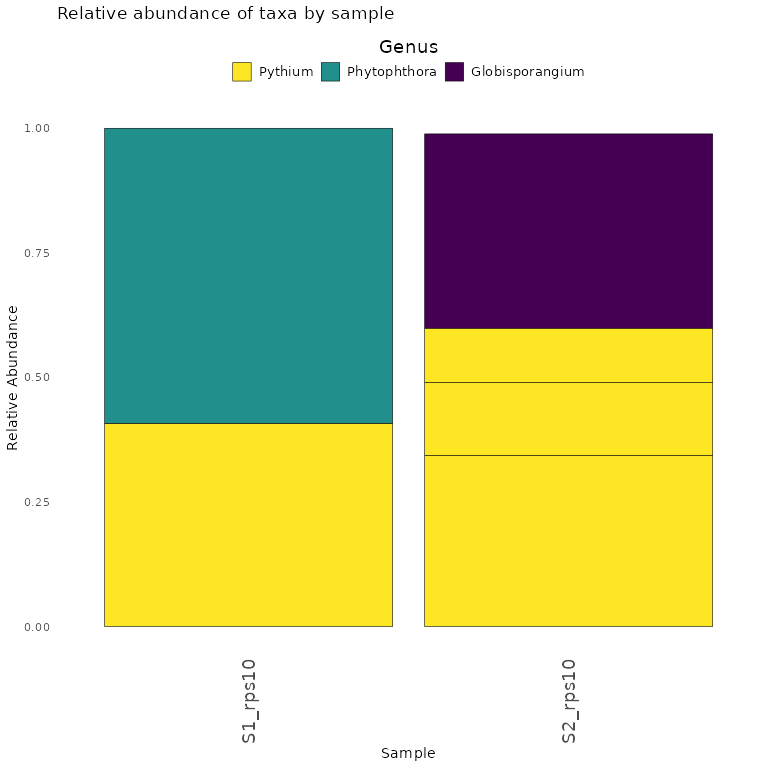
Finally, we demonstrate how to make a stacked bar plot of the relative abundance of taxa by sample for the rps10-barcoded samples

data <- objs$phyloseq_rps10 %>%
  phyloseq::transform_sample_counts(function(x) {x/sum(x)} ) %>% 
  phyloseq::psmelt() %>%                                        
  dplyr::filter(Abundance > 0.02) %>%                      
  dplyr::arrange(Genus)                                      

abund_plot <- ggplot2::ggplot(data, ggplot2::aes(x = Sample, y = Abundance, fill = Genus)) + 
  ggplot2::geom_bar(stat = "identity", position = "stack", color = "black", size = 0.2) +
  ggplot2::scale_fill_viridis_d() +
  ggplot2::theme_minimal() +
  ggplot2::labs(
    y = "Relative Abundance",
    title = "Relative abundance of taxa by sample",
    fill = "Genus"
  ) +
  ggplot2::theme(
    axis.text.x = ggplot2::element_text(angle = 90, hjust = 1, vjust = 0.5, size = 14),
    panel.grid.major = ggplot2::element_blank(),
    panel.grid.minor = ggplot2::element_blank(),
    legend.position = "top",
    legend.text = ggplot2::element_text(size = 14),
    legend.title = ggplot2::element_text(size = 14),  # Adjust legend title size
    strip.text = ggplot2::element_text(size = 14),
    strip.background = ggplot2::element_blank()
  ) +
  ggplot2::guides(
    fill = ggplot2::guide_legend(
      reverse = TRUE,
      keywidth = 1,
      keyheight = 1,
      title.position = "top",
      title.hjust = 0.5,  # Center the legend title
      label.theme = ggplot2::element_text(size = 10)  # Adjust the size of the legend labels
    )
  )

print(abund_plot)