Demonstration of how to use demulticoder on a dataset that is actually three separate datasets (RPS10, ITS, and 16S) at once
This is a small dataset comprised 24 samples. In three separate experiments, 16S, ITS, and 16S genes/regions were amplified, following an experiment in which some soil samples were treated with diallyl disulfide (organosulfur biocontrol compound derived from garlic), half were exposed to anaerobic conditions vs. aerobic conditions, and half the samples were one soil type (Tulelake) vs. another (Madras). The goal was to examine the bacterial, fungal, and oomycete communities within these different treatment groups. Reads were obtained following three separate Illumina MiSeq runs. The following Demulticoder workflow below picks up after these runs. The read data has already been demultiplexed, and for each sample, there is 16S, ITS, and rps10 reads within three separate FASTQ files per sample.
The goal of this workflow is to demonstrate that you can analyze simultaneously (but with different parameters), multiple datasets, related or not. Final matrices are separated by barcode, to avoid any violation of assumptions regarding experimental design. If the user so desires, they could combine the final matrices, depending on how the experiment was designed.
Step 1-Prepare metadata.csv file
You will see that sample names are unique for Here is the CSV file looks like:
sample_name,primer_name,incubation,soil,treatment
1_1_01,r16S,Anaerobic,Madras,untreated
1_2_01,r16S,Anaerobic,Madras,untreated
1_3_01,r16S,Anaerobic,Madras,untreated
2_1_01,r16S,Anaerobic,Madras,DADS_1gal_A
2_2_01,r16S,Anaerobic,Madras,DADS_1gal_A
2_3_01,r16S,Anaerobic,Madras,DADS_1gal_A
3_1_01,r16S,Anaerobic,Tulelake,untreated
3_2_01,r16S,Anaerobic,Tulelake,untreated
3_3_01,r16S,Anaerobic,Tulelake,untreated
4_1_01,r16S,Anaerobic,Tulelake,DADS_1gal_A
4_2_01,r16S,Anaerobic,Tulelake,DADS_1gal_A
4_3_01,r16S,Anaerobic,Tulelake,DADS_1gal_A
5_1_01,r16S,Aerobic,Madras,untreated
5_2_01,r16S,Aerobic,Madras,untreated
5_3_01,r16S,Aerobic,Madras,untreated
6_1_01,r16S,Aerobic,Madras,DADS_1gal_A
6_2_01,r16S,Aerobic,Madras,DADS_1gal_A
6_3_01,r16S,Aerobic,Madras,DADS_1gal_A
7_1_01,r16S,Aerobic,Tulelake,untreated
7_2_01,r16S,Aerobic,Tulelake,untreated
7_3_01,r16S,Aerobic,Tulelake,untreated
8_1_01,r16S,Aerobic,Tulelake,DADS_1gal_A
8_2_01,r16S,Aerobic,Tulelake,DADS_1gal_A
8_3_01,r16S,Aerobic,Tulelake,DADS_1gal_A
Dung1_1_S221_L001_02,its,Anaerobic ,Madras,untreated
Dung1_1_S222,rps10,Anaerobic ,Madras,untreated
Dung1_2_S222_L001_02,its,Anaerobic ,Madras,untreated
Dung1_2_S223,rps10,Anaerobic ,Madras,DADS_1gal_A
Dung1_3_S223_L001_02,its,Anaerobic ,Madras,DADS_1gal_A
Dung1_3_S224,rps10,Anaerobic ,Madras,DADS_1gal_A
Dung2_1_S224_L001_02,its,Anaerobic ,Tulelake,untreated
Dung2_1_S225,rps10,Anaerobic ,Tulelake,untreated
Dung2_2_S225_L001_02,its,Anaerobic ,Tulelake,untreated
Dung2_2_S226,rps10,Anaerobic ,Tulelake,DADS_1gal_A
Dung2_3_S226_L001_02,its,Anaerobic ,Tulelake,DADS_1gal_A
Dung2_3_S227,rps10,Anaerobic ,Tulelake,DADS_1gal_A
Dung3_1_S227_L001_02,its,Aerobic,Madras,untreated
Dung3_1_S228,rps10,Aerobic,Madras,untreated
Dung3_2_S228_L001_02,its,Aerobic,Madras,untreated
Dung3_2_S229,rps10,Aerobic,Madras,DADS_1gal_A
Dung3_3_S229_L001_02,its,Aerobic,Madras,DADS_1gal_A
Dung3_3_S230,rps10,Aerobic,Madras,DADS_1gal_A
Dung4_1_S230_L001_02,its,Aerobic,Tulelake,untreated
Dung4_1_S231,rps10,Aerobic,Tulelake,untreated
Dung4_2_S231_L001_02,its,Aerobic,Tulelake,untreated
Dung4_2_S232,rps10,Aerobic,Tulelake,DADS_1gal_A
Dung4_3_S232_L001_02,its,Aerobic,Tulelake,DADS_1gal_A
Dung4_3_S233,rps10,Aerobic,Tulelake,DADS_1gal_A
Dung5_1_S233_L001_02,its,Anaerobic ,Madras,untreated
Dung5_1_S234,rps10,Anaerobic ,Madras,untreated
Dung5_2_S234_L001_02,its,Anaerobic ,Madras,untreated
Dung5_2_S235,rps10,Anaerobic ,Madras,DADS_1gal_A
Dung5_3_S235_L001_02,its,Anaerobic ,Madras,DADS_1gal_A
Dung5_3_S236,rps10,Anaerobic ,Madras,DADS_1gal_A
Dung6_1_S236_L001_02,its,Anaerobic ,Tulelake,untreated
Dung6_1_S237,rps10,Anaerobic ,Tulelake,untreated
Dung6_2_S237_L001_02,its,Anaerobic ,Tulelake,untreated
Dung6_2_S238,rps10,Anaerobic ,Tulelake,DADS_1gal_A
Dung6_3_S238_L001_02,its,Anaerobic ,Tulelake,DADS_1gal_A
Dung6_3_S239,rps10,Anaerobic ,Tulelake,DADS_1gal_A
Dung7_1_S239_L001_02,its,Aerobic,Madras,untreated
Dung7_1_S240,rps10,Aerobic,Madras,untreated
Dung7_2_S240_L001_02,its,Aerobic,Madras,untreated
Dung7_2_S241,rps10,Aerobic,Madras,DADS_1gal_A
Dung7_3_S241_L001_02,its,Aerobic,Madras,DADS_1gal_A
Dung7_3_S242,rps10,Aerobic,Madras,DADS_1gal_A
Dung8_1_S242_L001_02,its,Aerobic,Tulelake,untreated
Dung8_1_S243,rps10,Aerobic,Tulelake,untreated
Dung8_2_S243_L001_02,its,Aerobic,Tulelake,untreated
Dung8_2_S244,rps10,Aerobic,Tulelake,DADS_1gal_A
Dung8_3_S244_L001_02,its,Aerobic,Tulelake,DADS_1gal_A
Dung8_3_S245,rps10,Aerobic,Tulelake,DADS_1gal_A
In tabular format:
| sample_name | primer_name | incubation | soil | treatment |
|---|---|---|---|---|
| 1_1_01 | r16S | Anaerobic | Madras | untreated |
| 1_2_01 | r16S | Anaerobic | Madras | untreated |
| 1_3_01 | r16S | Anaerobic | Madras | untreated |
| 2_1_01 | r16S | Anaerobic | Madras | DADS_1gal_A |
| 2_2_01 | r16S | Anaerobic | Madras | DADS_1gal_A |
| 2_3_01 | r16S | Anaerobic | Madras | DADS_1gal_A |
| 3_1_01 | r16S | Anaerobic | Tulelake | untreated |
| 3_2_01 | r16S | Anaerobic | Tulelake | untreated |
| 3_3_01 | r16S | Anaerobic | Tulelake | untreated |
| 4_1_01 | r16S | Anaerobic | Tulelake | DADS_1gal_A |
| 4_2_01 | r16S | Anaerobic | Tulelake | DADS_1gal_A |
| 4_3_01 | r16S | Anaerobic | Tulelake | DADS_1gal_A |
| 5_1_01 | r16S | Aerobic | Madras | untreated |
| 5_2_01 | r16S | Aerobic | Madras | untreated |
| 5_3_01 | r16S | Aerobic | Madras | untreated |
| 6_1_01 | r16S | Aerobic | Madras | DADS_1gal_A |
| 6_2_01 | r16S | Aerobic | Madras | DADS_1gal_A |
| 6_3_01 | r16S | Aerobic | Madras | DADS_1gal_A |
| 7_1_01 | r16S | Aerobic | Tulelake | untreated |
| 7_2_01 | r16S | Aerobic | Tulelake | untreated |
| 7_3_01 | r16S | Aerobic | Tulelake | untreated |
| 8_1_01 | r16S | Aerobic | Tulelake | DADS_1gal_A |
| 8_2_01 | r16S | Aerobic | Tulelake | DADS_1gal_A |
| 8_3_01 | r16S | Aerobic | Tulelake | DADS_1gal_A |
Step 2-Prepare primerinfo_params.csv file
Here is the CSV file looks like:
primer_name,forward,reverse,already_trimmed,minCutadaptlength,multithread,verbose,maxN,maxEE_forward,maxEE_reverse,truncLen_forward,truncLen_reverse,truncQ,minLen,maxLen,minQ,trimLeft,trimRight,rm.lowcomplex,minOverlap,maxMismatch,min_asv_length
rps10,GTTGGTTAGAGYARAAGACT,ATRYYTAGAAAGAYTYGAACT,FALSE,50,TRUE,TRUE,0,5,5,0,0,5,50,Inf,0,0,0,0,15,2,50
its,GTGARTCATCGAATCTTTG,TCCTSCGCTTATTGATATGC,FALSE,50,TRUE,TRUE,0,2,2,0,0,5,50,295,0,0,0,0,15,2,50
r16S,GTGYCAGCMGCCGCGGTAA,GGACTACNVGGGTWTCTAAT,TRUE,50,TRUE,TRUE,0,2,2,0,0,5,50,Inf,0,0,0,0,15,2,50
In tabular format:
| primer_name | forward | reverse | already_trimmed | minCutadaptlength | multithread | verbose | maxN | maxEE_forward | maxEE_reverse | truncLen_forward | truncLen_reverse | truncQ | minLen | maxLen | minQ | trimLeft | trimRight | rm.lowcomplex | minOverlap | maxMismatch | min_asv_length |
|---|---|---|---|---|---|---|---|---|---|---|---|---|---|---|---|---|---|---|---|---|---|
| rps10 | GTTGGTTAGAGYARAAGACT | ATRYYTAGAAAGAYTYGAACT | FALSE | 50 | TRUE | TRUE | 0 | 5 | 5 | 0 | 0 | 5 | 50 | Inf | 0 | 0 | 0 | 0 | 15 | 2 | 50 |
| its | GTGARTCATCGAATCTTTG | TCCTSCGCTTATTGATATGC | FALSE | 50 | TRUE | TRUE | 0 | 2 | 2 | 0 | 0 | 5 | 50 | 295 | 0 | 0 | 0 | 0 | 15 | 2 | 50 |
| r16S | GTGYCAGCMGCCGCGGTAA | GGACTACNVGGGTWTCTAAT | TRUE | 50 | TRUE | TRUE | 0 | 2 | 2 | 0 | 0 | 5 | 50 | Inf | 0 | 0 | 0 | 0 | 15 | 2 | 50 |
Step 3-Remove N’s and create directory structure for downstream steps
outputs<-prepare_reads(
data_directory = "~/demulticoder_benchmarking/demulticoder_combined_analysis_dads/data",
output_directory = "~/demulticoder_benchmarking/package_vignettes/output_multiple_datasets",
tempdir_path = "~/demulticoder_benchmarking/temp",
overwrite_existing = TRUE)
#> Rows: 3 Columns: 22
#> ── Column specification ────────────────────────────────────────────────────────
#> Delimiter: ","
#> chr (3): primer_name, forward, reverse
#> dbl (16): minCutadaptlength, maxN, maxEE_forward, maxEE_reverse, truncLen_fo...
#> lgl (3): already_trimmed, multithread, verbose
#>
#> ℹ Use `spec()` to retrieve the full column specification for this data.
#> ℹ Specify the column types or set `show_col_types = FALSE` to quiet this message.
#> Rows: 72 Columns: 5
#> ── Column specification ────────────────────────────────────────────────────────
#> Delimiter: ","
#> chr (5): sample_name, primer_name, incubation, soil, treatment
#>
#> ℹ Use `spec()` to retrieve the full column specification for this data.
#> ℹ Specify the column types or set `show_col_types = FALSE` to quiet this message.
#> Creating output directory: /home/marthasudermann/demulticoder_benchmarking/temp/demulticoder_run/prefiltered_sequences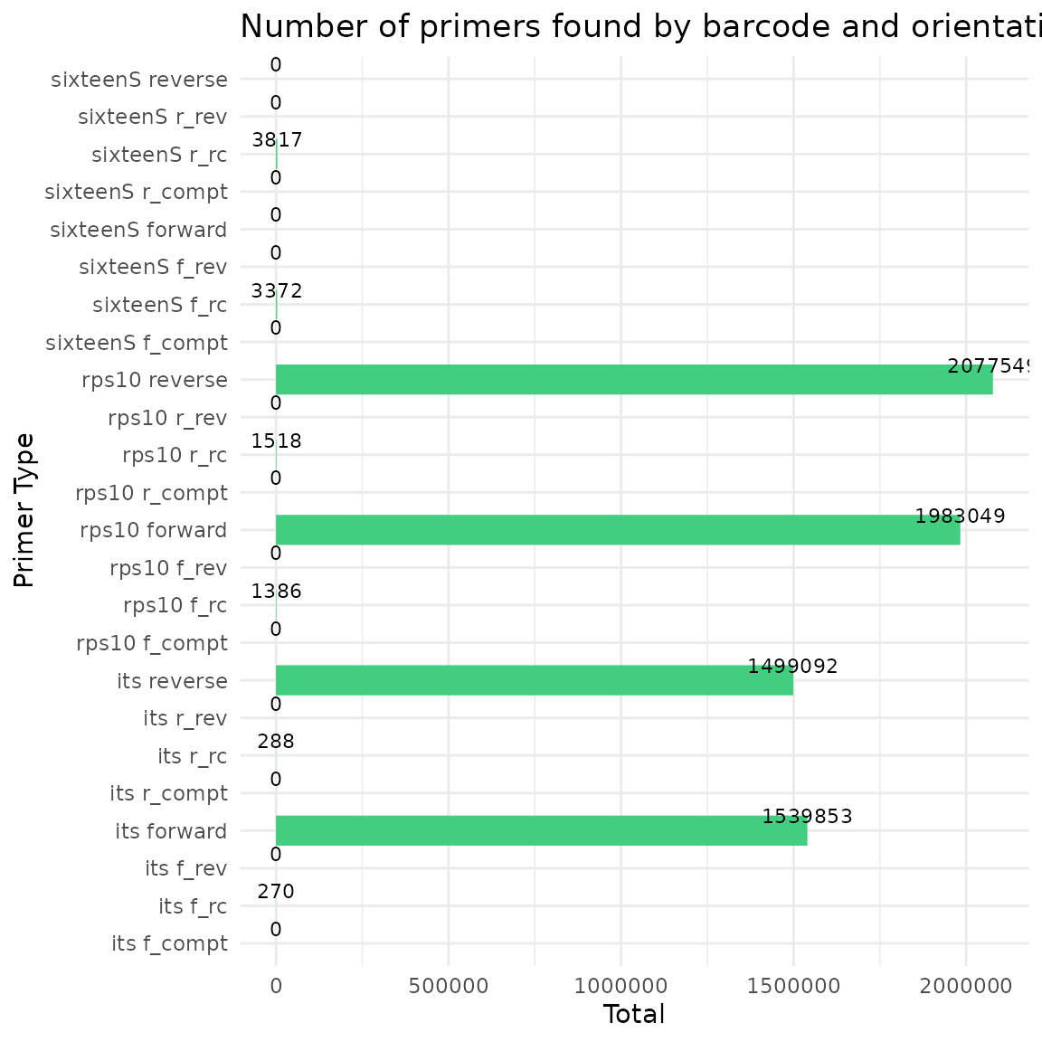
Step 4-Run Cutadapt to remove primers and then trim reads with DADA2 filterAndTrim function
cut_trim(
  outputs,
  cutadapt_path="/usr/bin/cutadapt",
  overwrite_existing = TRUE)
#> Running Cutadapt 3.5 for its sequence data
#> Running Cutadapt 3.5 for rps10 sequence data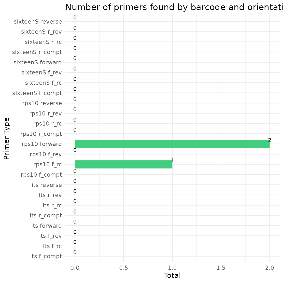
Step 5-Core ASV inference step
make_asv_abund_matrix(
  outputs,
  overwrite_existing = TRUE)
#> 106034910 total bases in 466183 reads from 9 samples will be used for learning the error rates.
#> Initializing error rates to maximum possible estimate.
#> selfConsist step 1 .........
#>    selfConsist step 2
#>    selfConsist step 3
#>    selfConsist step 4
#>    selfConsist step 5
#> Convergence after  5  rounds.
#> Error rate plot for the Forward read of primer pair its
#> Warning in scale_y_log10(): log-10 transformation introduced
#> infinite values.
#> Sample 1 - 78090 reads in 14475 unique sequences.
#> Sample 2 - 45955 reads in 9604 unique sequences.
#> Sample 3 - 42450 reads in 9362 unique sequences.
#> Sample 4 - 47513 reads in 13905 unique sequences.
#> Sample 5 - 37652 reads in 12257 unique sequences.
#> Sample 6 - 50196 reads in 15866 unique sequences.
#> Sample 7 - 33726 reads in 7781 unique sequences.
#> Sample 8 - 48490 reads in 10219 unique sequences.
#> Sample 9 - 82111 reads in 14763 unique sequences.
#> Sample 10 - 65012 reads in 18955 unique sequences.
#> Sample 11 - 50432 reads in 13490 unique sequences.
#> Sample 12 - 44904 reads in 13902 unique sequences.
#> Sample 13 - 35611 reads in 7806 unique sequences.
#> Sample 14 - 29981 reads in 7103 unique sequences.
#> Sample 15 - 35426 reads in 8032 unique sequences.
#> Sample 16 - 40535 reads in 13049 unique sequences.
#> Sample 17 - 37788 reads in 11717 unique sequences.
#> Sample 18 - 25282 reads in 8508 unique sequences.
#> Sample 19 - 24576 reads in 5694 unique sequences.
#> Sample 20 - 31335 reads in 7645 unique sequences.
#> Sample 21 - 37061 reads in 7258 unique sequences.
#> Sample 22 - 30407 reads in 9859 unique sequences.
#> Sample 23 - 42100 reads in 11928 unique sequences.
#> Sample 24 - 57989 reads in 16385 unique sequences.
#> 105499828 total bases in 466183 reads from 9 samples will be used for learning the error rates.
#> Initializing error rates to maximum possible estimate.
#> selfConsist step 1 .........
#>    selfConsist step 2
#>    selfConsist step 3
#>    selfConsist step 4
#> Convergence after  4  rounds.
#> Error rate plot for the Reverse read of primer pair its
#> Warning in scale_y_log10(): log-10 transformation introduced
#> infinite values.
#> Sample 1 - 78090 reads in 18561 unique sequences.
#> Sample 2 - 45955 reads in 11830 unique sequences.
#> Sample 3 - 42450 reads in 12227 unique sequences.
#> Sample 4 - 47513 reads in 12720 unique sequences.
#> Sample 5 - 37652 reads in 15089 unique sequences.
#> Sample 6 - 50196 reads in 19051 unique sequences.
#> Sample 7 - 33726 reads in 12311 unique sequences.
#> Sample 8 - 48490 reads in 17792 unique sequences.
#> Sample 9 - 82111 reads in 19363 unique sequences.
#> Sample 10 - 65012 reads in 16307 unique sequences.
#> Sample 11 - 50432 reads in 12229 unique sequences.
#> Sample 12 - 44904 reads in 12850 unique sequences.
#> Sample 13 - 35611 reads in 9856 unique sequences.
#> Sample 14 - 29981 reads in 8435 unique sequences.
#> Sample 15 - 35426 reads in 10431 unique sequences.
#> Sample 16 - 40535 reads in 10489 unique sequences.
#> Sample 17 - 37788 reads in 18061 unique sequences.
#> Sample 18 - 25282 reads in 11321 unique sequences.
#> Sample 19 - 24576 reads in 13200 unique sequences.
#> Sample 20 - 31335 reads in 13584 unique sequences.
#> Sample 21 - 37061 reads in 10363 unique sequences.
#> Sample 22 - 30407 reads in 9253 unique sequences.
#> Sample 23 - 42100 reads in 10947 unique sequences.
#> Sample 24 - 57989 reads in 13634 unique sequences.
#> 76532 paired-reads (in 235 unique pairings) successfully merged out of 77154 (in 268 pairings) input.
#> Duplicate sequences in merged output.
#> 44826 paired-reads (in 182 unique pairings) successfully merged out of 45262 (in 211 pairings) input.
#> Duplicate sequences in merged output.
#> 41241 paired-reads (in 177 unique pairings) successfully merged out of 41588 (in 200 pairings) input.
#> Duplicate sequences in merged output.
#> 46443 paired-reads (in 134 unique pairings) successfully merged out of 46791 (in 153 pairings) input.
#> Duplicate sequences in merged output.
#> 36763 paired-reads (in 118 unique pairings) successfully merged out of 36988 (in 133 pairings) input.
#> Duplicate sequences in merged output.
#> 49327 paired-reads (in 138 unique pairings) successfully merged out of 49592 (in 153 pairings) input.
#> Duplicate sequences in merged output.
#> 32710 paired-reads (in 136 unique pairings) successfully merged out of 33009 (in 158 pairings) input.
#> Duplicate sequences in merged output.
#> 47112 paired-reads (in 167 unique pairings) successfully merged out of 47654 (in 200 pairings) input.
#> Duplicate sequences in merged output.
#> 80706 paired-reads (in 239 unique pairings) successfully merged out of 81276 (in 280 pairings) input.
#> Duplicate sequences in merged output.
#> 63826 paired-reads (in 177 unique pairings) successfully merged out of 64176 (in 202 pairings) input.
#> Duplicate sequences in merged output.
#> 49621 paired-reads (in 117 unique pairings) successfully merged out of 49737 (in 131 pairings) input.
#> Duplicate sequences in merged output.
#> 43962 paired-reads (in 136 unique pairings) successfully merged out of 44349 (in 154 pairings) input.
#> Duplicate sequences in merged output.
#> 34455 paired-reads (in 154 unique pairings) successfully merged out of 34905 (in 181 pairings) input.
#> Duplicate sequences in merged output.
#> 28736 paired-reads (in 155 unique pairings) successfully merged out of 29390 (in 181 pairings) input.
#> Duplicate sequences in merged output.
#> 33960 paired-reads (in 163 unique pairings) successfully merged out of 34687 (in 188 pairings) input.
#> Duplicate sequences in merged output.
#> 39776 paired-reads (in 129 unique pairings) successfully merged out of 39921 (in 142 pairings) input.
#> Duplicate sequences in merged output.
#> 36836 paired-reads (in 104 unique pairings) successfully merged out of 36988 (in 113 pairings) input.
#> Duplicate sequences in merged output.
#> 24650 paired-reads (in 88 unique pairings) successfully merged out of 24794 (in 96 pairings) input.
#> Duplicate sequences in merged output.
#> 23672 paired-reads (in 102 unique pairings) successfully merged out of 23918 (in 118 pairings) input.
#> Duplicate sequences in merged output.
#> 30099 paired-reads (in 103 unique pairings) successfully merged out of 30492 (in 123 pairings) input.
#> Duplicate sequences in merged output.
#> 35951 paired-reads (in 148 unique pairings) successfully merged out of 36386 (in 166 pairings) input.
#> Duplicate sequences in merged output.
#> 29757 paired-reads (in 117 unique pairings) successfully merged out of 29919 (in 126 pairings) input.
#> Duplicate sequences in merged output.
#> 41280 paired-reads (in 143 unique pairings) successfully merged out of 41588 (in 162 pairings) input.
#> Duplicate sequences in merged output.
#> 56900 paired-reads (in 156 unique pairings) successfully merged out of 57408 (in 180 pairings) input.
#> Duplicate sequences in merged output.
#> Duplicate sequences detected and merged.
#> Duplicate sequences detected and merged.
#> Duplicate sequences detected and merged.
#> Duplicate sequences detected and merged.
#> Duplicate sequences detected and merged.
#> Duplicate sequences detected and merged.
#> Duplicate sequences detected and merged.
#> Duplicate sequences detected and merged.
#> Duplicate sequences detected and merged.
#> Duplicate sequences detected and merged.
#> Duplicate sequences detected and merged.
#> Duplicate sequences detected and merged.
#> Duplicate sequences detected and merged.
#> Duplicate sequences detected and merged.
#> Duplicate sequences detected and merged.
#> Duplicate sequences detected and merged.
#> Duplicate sequences detected and merged.
#> Duplicate sequences detected and merged.
#> Duplicate sequences detected and merged.
#> Duplicate sequences detected and merged.
#> Duplicate sequences detected and merged.
#> Duplicate sequences detected and merged.
#> Duplicate sequences detected and merged.
#> Duplicate sequences detected and merged.
#> Identified 28 bimeras out of 869 input sequences.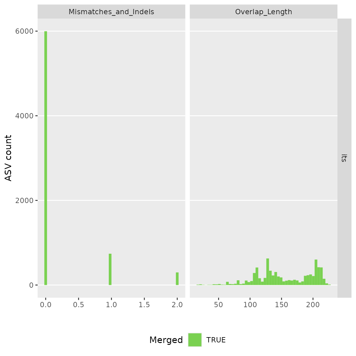
#> 126787839 total bases in 451263 reads from 6 samples will be used for learning the error rates.
#> Initializing error rates to maximum possible estimate.
#> selfConsist step 1 ......
#>    selfConsist step 2
#>    selfConsist step 3
#>    selfConsist step 4
#>    selfConsist step 5
#> Convergence after  5  rounds.
#> Error rate plot for the Forward read of primer pair rps10
#> Sample 1 - 20082 reads in 15404 unique sequences.
#> Sample 2 - 81794 reads in 50235 unique sequences.
#> Sample 3 - 86486 reads in 57261 unique sequences.
#> Sample 4 - 64939 reads in 48091 unique sequences.
#> Sample 5 - 79738 reads in 50805 unique sequences.
#> Sample 6 - 118224 reads in 69385 unique sequences.
#> Sample 7 - 19427 reads in 13201 unique sequences.
#> Sample 8 - 73752 reads in 47699 unique sequences.
#> Sample 9 - 23829 reads in 16766 unique sequences.
#> Sample 10 - 69370 reads in 41438 unique sequences.
#> Sample 11 - 134589 reads in 79909 unique sequences.
#> Sample 12 - 88315 reads in 55387 unique sequences.
#> Sample 13 - 43607 reads in 37646 unique sequences.
#> Sample 14 - 68342 reads in 51601 unique sequences.
#> Sample 15 - 14251 reads in 12014 unique sequences.
#> Sample 16 - 10633 reads in 9740 unique sequences.
#> Sample 17 - 99725 reads in 58227 unique sequences.
#> Sample 18 - 82697 reads in 49568 unique sequences.
#> Sample 19 - 58679 reads in 39009 unique sequences.
#> Sample 20 - 58661 reads in 40824 unique sequences.
#> Sample 21 - 46627 reads in 39317 unique sequences.
#> Sample 22 - 60360 reads in 46852 unique sequences.
#> Sample 23 - 14006 reads in 11814 unique sequences.
#> Sample 24 - 22369 reads in 18243 unique sequences.
#> 126347798 total bases in 451263 reads from 6 samples will be used for learning the error rates.
#> Initializing error rates to maximum possible estimate.
#> selfConsist step 1 ......
#>    selfConsist step 2
#>    selfConsist step 3
#>    selfConsist step 4
#>    selfConsist step 5
#>    selfConsist step 6
#>    selfConsist step 7
#> Convergence after  7  rounds.
#> Error rate plot for the Reverse read of primer pair rps10
#> Sample 1 - 20082 reads in 14654 unique sequences.
#> Sample 2 - 81794 reads in 56653 unique sequences.
#> Sample 3 - 86486 reads in 61939 unique sequences.
#> Sample 4 - 64939 reads in 41617 unique sequences.
#> Sample 5 - 79738 reads in 48181 unique sequences.
#> Sample 6 - 118224 reads in 71942 unique sequences.
#> Sample 7 - 19427 reads in 14744 unique sequences.
#> Sample 8 - 73752 reads in 53141 unique sequences.
#> Sample 9 - 23829 reads in 17238 unique sequences.
#> Sample 10 - 69370 reads in 41800 unique sequences.
#> Sample 11 - 134589 reads in 73468 unique sequences.
#> Sample 12 - 88315 reads in 51668 unique sequences.
#> Sample 13 - 43607 reads in 29142 unique sequences.
#> Sample 14 - 68342 reads in 42353 unique sequences.
#> Sample 15 - 14251 reads in 10551 unique sequences.
#> Sample 16 - 10633 reads in 6488 unique sequences.
#> Sample 17 - 99725 reads in 56068 unique sequences.
#> Sample 18 - 82697 reads in 47196 unique sequences.
#> Sample 19 - 58679 reads in 43743 unique sequences.
#> Sample 20 - 58661 reads in 40142 unique sequences.
#> Sample 21 - 46627 reads in 33507 unique sequences.
#> Sample 22 - 60360 reads in 31906 unique sequences.
#> Sample 23 - 14006 reads in 8796 unique sequences.
#> Sample 24 - 22369 reads in 13421 unique sequences.
#> 19680 paired-reads (in 36 unique pairings) successfully merged out of 19998 (in 91 pairings) input.
#> Duplicate sequences in merged output.
#> 77741 paired-reads (in 72 unique pairings) successfully merged out of 81624 (in 162 pairings) input.
#> Duplicate sequences in merged output.
#> 81094 paired-reads (in 72 unique pairings) successfully merged out of 86377 (in 191 pairings) input.
#> Duplicate sequences in merged output.
#> 60693 paired-reads (in 192 unique pairings) successfully merged out of 64495 (in 586 pairings) input.
#> Duplicate sequences in merged output.
#> 75768 paired-reads (in 125 unique pairings) successfully merged out of 79396 (in 371 pairings) input.
#> Duplicate sequences in merged output.
#> 113422 paired-reads (in 172 unique pairings) successfully merged out of 117935 (in 471 pairings) input.
#> Duplicate sequences in merged output.
#> 18957 paired-reads (in 42 unique pairings) successfully merged out of 19137 (in 78 pairings) input.
#> Duplicate sequences in merged output.
#> 70795 paired-reads (in 79 unique pairings) successfully merged out of 73418 (in 146 pairings) input.
#> Duplicate sequences in merged output.
#> 23206 paired-reads (in 26 unique pairings) successfully merged out of 23760 (in 54 pairings) input.
#> Duplicate sequences in merged output.
#> 66712 paired-reads (in 81 unique pairings) successfully merged out of 69287 (in 241 pairings) input.
#> Duplicate sequences in merged output.
#> 128424 paired-reads (in 143 unique pairings) successfully merged out of 134179 (in 349 pairings) input.
#> Duplicate sequences in merged output.
#> 85426 paired-reads (in 85 unique pairings) successfully merged out of 88207 (in 264 pairings) input.
#> Duplicate sequences in merged output.
#> 41456 paired-reads (in 37 unique pairings) successfully merged out of 43409 (in 115 pairings) input.
#> Duplicate sequences in merged output.
#> 65184 paired-reads (in 84 unique pairings) successfully merged out of 68075 (in 205 pairings) input.
#> Duplicate sequences in merged output.
#> 13965 paired-reads (in 31 unique pairings) successfully merged out of 14174 (in 66 pairings) input.
#> Duplicate sequences in merged output.
#> 9229 paired-reads (in 16 unique pairings) successfully merged out of 10463 (in 76 pairings) input.
#> Duplicate sequences in merged output.
#> 96759 paired-reads (in 63 unique pairings) successfully merged out of 99648 (in 198 pairings) input.
#> Duplicate sequences in merged output.
#> 78760 paired-reads (in 80 unique pairings) successfully merged out of 82349 (in 244 pairings) input.
#> Duplicate sequences in merged output.
#> 52961 paired-reads (in 106 unique pairings) successfully merged out of 58370 (in 267 pairings) input.
#> Duplicate sequences in merged output.
#> 52492 paired-reads (in 81 unique pairings) successfully merged out of 58507 (in 209 pairings) input.
#> Duplicate sequences in merged output.
#> 44849 paired-reads (in 60 unique pairings) successfully merged out of 45994 (in 190 pairings) input.
#> Duplicate sequences in merged output.
#> 58198 paired-reads (in 55 unique pairings) successfully merged out of 60194 (in 175 pairings) input.
#> Duplicate sequences in merged output.
#> 13004 paired-reads (in 19 unique pairings) successfully merged out of 13817 (in 65 pairings) input.
#> 21168 paired-reads (in 38 unique pairings) successfully merged out of 22205 (in 167 pairings) input.
#> Duplicate sequences in merged output.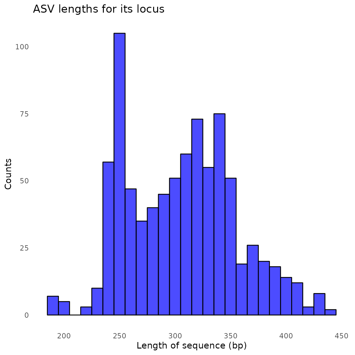
#> Duplicate sequences detected and merged.
#> Duplicate sequences detected and merged.
#> Duplicate sequences detected and merged.
#> Duplicate sequences detected and merged.
#> Duplicate sequences detected and merged.
#> Duplicate sequences detected and merged.
#> Duplicate sequences detected and merged.
#> Duplicate sequences detected and merged.
#> Duplicate sequences detected and merged.
#> Duplicate sequences detected and merged.
#> Duplicate sequences detected and merged.
#> Duplicate sequences detected and merged.
#> Duplicate sequences detected and merged.
#> Duplicate sequences detected and merged.
#> Duplicate sequences detected and merged.
#> Duplicate sequences detected and merged.
#> Duplicate sequences detected and merged.
#> Duplicate sequences detected and merged.
#> Duplicate sequences detected and merged.
#> Duplicate sequences detected and merged.
#> Duplicate sequences detected and merged.
#> Duplicate sequences detected and merged.
#> Duplicate sequences detected and merged.
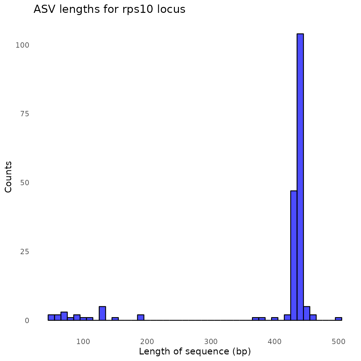
#> Identified 548 bimeras out of 732 input sequences.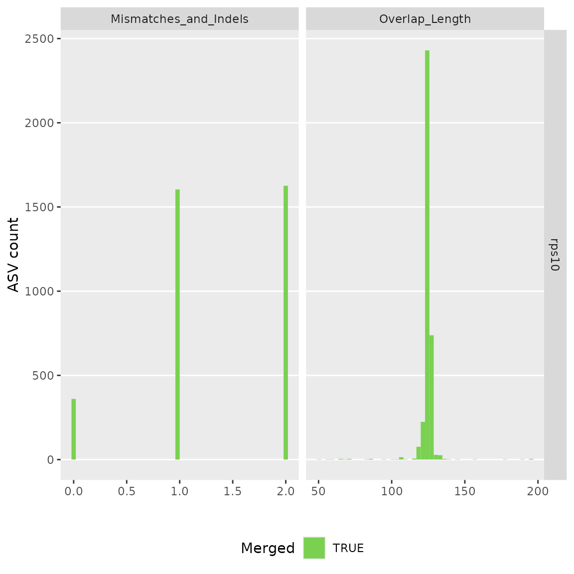
#> $its
#> [1] "~/demulticoder_benchmarking/temp/demulticoder_run/asvabund_matrixDADA2_its.RData"
#>
#> $rps10
#> [1] "~/demulticoder_benchmarking/temp/demulticoder_run/asvabund_matrixDADA2_rps10.RData"
Step 6-Assign taxonomy step
assign_tax(
  outputs,
  asv_abund_matrix,
  db_its = "sh_general_release_dynamic_all_25.07.2023.fasta",
  db_rps10 = "oomycetedb.fasta",
  db_16S="silva_nr99_v138.1_wSpecies_train_set.fa",
  retrieve_files=TRUE,
  overwrite_existing=TRUE)
#> Duplicate sequences detected and merged.
#> Duplicate sequences detected and merged.
#> Duplicate sequences detected and merged.
#> Duplicate sequences detected and merged.
#> Duplicate sequences detected and merged.
#> Duplicate sequences detected and merged.
#> Duplicate sequences detected and merged.
#> Duplicate sequences detected and merged.
#> Duplicate sequences detected and merged.
#> Duplicate sequences detected and merged.
#> Duplicate sequences detected and merged.
#> Duplicate sequences detected and merged.
#> Duplicate sequences detected and merged.
#> Duplicate sequences detected and merged.
#> Duplicate sequences detected and merged.
#> Duplicate sequences detected and merged.
#> Duplicate sequences detected and merged.
#> Duplicate sequences detected and merged.
#> Duplicate sequences detected and merged.
#> Duplicate sequences detected and merged.
#> Duplicate sequences detected and merged.
#> Duplicate sequences detected and merged.
#> Duplicate sequences detected and merged.
#> Duplicate sequences detected and merged.
#>          samplename_barcode  input filtered denoisedF denoisedR merged nonchim
#> 1  Dung1_1_S221_L001_02_its 107502    78090     77364     77495  76532   76477
#> 2  Dung1_2_S222_L001_02_its  61061    45955     45480     45404  44826   44775
#> 3  Dung1_3_S223_L001_02_its  61239    42450     41879     41813  41241   41212
#> 4  Dung2_1_S224_L001_02_its  63088    47513     47053     46978  46443   46146
#> 5  Dung2_2_S225_L001_02_its  58055    37652     37262     37094  36763   36571
#> 6  Dung2_3_S226_L001_02_its  80809    50196     49877     49673  49327   49046
#> 7  Dung3_1_S227_L001_02_its  52495    33726     33220     33165  32710   32681
#> 8  Dung3_2_S228_L001_02_its  81501    48490     48003     47784  47112   47069
#> 9  Dung3_3_S229_L001_02_its 109828    82111     81638     81435  80706   80549
#> 10 Dung4_1_S230_L001_02_its  89140    65012     64527     64413  63826   63378
#> 11 Dung4_2_S231_L001_02_its  63345    50432     49931     49931  49621   49267
#> 12 Dung4_3_S232_L001_02_its  59459    44904     44543     44470  43962   43633
#> 13 Dung5_1_S233_L001_02_its  46202    35611     35150     35057  34455   34400
#> 14 Dung5_2_S234_L001_02_its  39533    29981     29579     29519  28736   28722
#> 15 Dung5_3_S235_L001_02_its  56309    35426     34922     34913  33960   33933
#> 16 Dung6_1_S236_L001_02_its  54091    40535     40136     40108  39776   39536
#> 17 Dung6_2_S237_L001_02_its  83307    37788     37413     37100  36836   36644
#> 18 Dung6_3_S238_L001_02_its  49829    25282     24998     24834  24650   24515
#> 19 Dung7_1_S239_L001_02_its  57541    24576     24220     23984  23672   23652
#> 20 Dung7_2_S240_L001_02_its  54654    31335     30784     30639  30099   30043
#> 21 Dung7_3_S241_L001_02_its  49902    37061     36566     36567  35951   35934
#> 22 Dung8_1_S242_L001_02_its  42973    30407     30060     30025  29757   29561
#> 23 Dung8_2_S243_L001_02_its  58646    42100     41795     41701  41280   41090
#> 24 Dung8_3_S244_L001_02_its  77154    57989     57602     57554  56900   56623
#> Duplicate sequences detected and merged.
#> Duplicate sequences detected and merged.
#> Duplicate sequences detected and merged.
#> Duplicate sequences detected and merged.
#> Duplicate sequences detected and merged.
#> Duplicate sequences detected and merged.
#> Duplicate sequences detected and merged.
#> Duplicate sequences detected and merged.
#> Duplicate sequences detected and merged.
#> Duplicate sequences detected and merged.
#> Duplicate sequences detected and merged.
#> Duplicate sequences detected and merged.
#> Duplicate sequences detected and merged.
#> Duplicate sequences detected and merged.
#> Duplicate sequences detected and merged.
#> Duplicate sequences detected and merged.
#> Duplicate sequences detected and merged.
#> Duplicate sequences detected and merged.
#> Duplicate sequences detected and merged.
#> Duplicate sequences detected and merged.
#> Duplicate sequences detected and merged.
#> Duplicate sequences detected and merged.
#> Duplicate sequences detected and merged.
#>    samplename_barcode  input filtered denoisedF denoisedR merged nonchim
#> 1  Dung1_1_S222_rps10  31012    20082     19999     20028  19680   19259
#> 2  Dung1_2_S223_rps10 117900    81794     81719     81690  77741   75601
#> 3  Dung1_3_S224_rps10 132855    86486     86438     86422  81094   78814
#> 4  Dung2_1_S225_rps10  96066    64939     64784     64631  60693   48037
#> 5  Dung2_2_S226_rps10 111356    79738     79519     79577  75768   64714
#> 6  Dung2_3_S227_rps10 159936   118224    117976    118170 113422  100408
#> 7  Dung3_1_S228_rps10  28596    19427     19389     19156  18957   18414
#> 8  Dung3_2_S229_rps10 110053    73752     73617     73544  70795   66612
#> 9  Dung3_3_S230_rps10  35693    23829     23784     23793  23206   22878
#> 10 Dung4_1_S231_rps10  94160    69370     69320     69327  66712   63797
#> 11 Dung4_2_S232_rps10 181941   134589    134530    134227 128424  114055
#> 12 Dung4_3_S233_rps10 120075    88315     88238     88236  85426   79149
#> 13 Dung5_1_S234_rps10  89019    43607     43478     43503  41456   38404
#> 14 Dung5_2_S235_rps10 104996    68342     68208     68192  65184   58908
#> 15 Dung5_3_S236_rps10  25501    14251     14203     14187  13965   13760
#> 16 Dung6_1_S237_rps10  24523    10633     10478     10606   9229    8739
#> 17 Dung6_2_S238_rps10 147048    99725     99704     99664  96759   94361
#> 18 Dung6_3_S239_rps10 114844    82697     82620     82402  78760   74217
#> 19 Dung7_1_S240_rps10  86521    58679     58432     58604  52961   49033
#> 20 Dung7_2_S241_rps10  86204    58661     58550     58608  52492   48440
#> 21 Dung7_3_S242_rps10  90932    46627     46444     46136  44849   43436
#> 22 Dung8_1_S243_rps10  95078    60360     60213     60329  58198   54921
#> 23 Dung8_2_S244_rps10  23896    14006     13876     13927  13004   12520
#> 24 Dung8_3_S245_rps10  36871    22369     22225     22326  21168   20016
Step 7-convert asv matrix to taxmap and phyloseq objects with one function
objs<-convert_asv_matrix_to_objs(outputs, save_outputs=TRUE, overwrite_existing = TRUE)
#> Rows: 841 Columns: 27
#> ── Column specification ────────────────────────────────────────────────────────
#> Delimiter: ","
#> chr  (3): asv_id, sequence, dada2_tax
#> dbl (24): Dung1_1_S221_L001_02_its, Dung1_2_S222_L001_02_its, Dung1_3_S223_L...
#>
#> ℹ Use `spec()` to retrieve the full column specification for this data.
#> ℹ Specify the column types or set `show_col_types = FALSE` to quiet this message.
#> For its dataset
#> Taxmap object saved in: ~/demulticoder_benchmarking/package_vignettes/output_multiple_datasets/obj_dada_its.RData
#> Phyloseq object saved in: ~/demulticoder_benchmarking/package_vignettes/output_multiple_datasets/phylo_obj_its.RData
#> ASVs filtered by minimum read depth: 0
#> For taxonomic assignments, if minimum bootstrap was set to: 0 assignments were set to 'Unsupported'
#> ~~~~~~~~~~~~~~~~~~~~~~~~~~~~~~~~~~~~
#> Rows: 184 Columns: 27
#> ── Column specification ────────────────────────────────────────────────────────
#> Delimiter: ","
#> chr  (3): asv_id, sequence, dada2_tax
#> dbl (24): Dung1_1_S222_rps10, Dung1_2_S223_rps10, Dung1_3_S224_rps10, Dung2_...
#>
#> ℹ Use `spec()` to retrieve the full column specification for this data.
#> ℹ Specify the column types or set `show_col_types = FALSE` to quiet this message.
#> For rps10 dataset
#> Taxmap object saved in: ~/demulticoder_benchmarking/package_vignettes/output_multiple_datasets/obj_dada_rps10.RData
#> Phyloseq object saved in: ~/demulticoder_benchmarking/package_vignettes/output_multiple_datasets/phylo_obj_rps10.RData
#> ASVs filtered by minimum read depth: 0
#> For taxonomic assignments, if minimum bootstrap was set to: 0 assignments were set to 'Unsupported'
#> ~~~~~~~~~~~~~~~~~~~~~~~~~~~~~~~~~~~~
Use phyloseq objects to examine the community composition of each sample
Here we demonstrate how to make a stacked bar plot of the relative abundance of taxa by sample for the 16S-barcoded samples
data <- objs$phyloseq_its %>%
  phyloseq::transform_sample_counts(function(x) {x/sum(x)} ) %>%
  phyloseq::psmelt() %>%
  dplyr::filter(Abundance > 0.005) %>%
  dplyr::arrange(Genus)

abund_plot <- ggplot2::ggplot(data, ggplot2::aes(x = Sample, y = Abundance, fill = Genus)) +
  ggplot2::geom_bar(stat = "identity", position = "stack", color = "black", size = 0.2) +
  ggplot2::scale_fill_viridis_d() +
  ggplot2::theme_minimal() +
  ggplot2::labs(
    y = "Relative Abundance",
    title = "Relative abundance of taxa by sample",
    fill = "Genus"
  ) +
  ggplot2::theme(
    axis.text.x = ggplot2::element_text(angle = 90, hjust = 1, vjust = 0.5, size = 10),
    panel.grid.major = ggplot2::element_blank(),
    panel.grid.minor = ggplot2::element_blank(),
    legend.position = "top",
    legend.text = ggplot2::element_text(size = 10),
    legend.title = ggplot2::element_text(size = 10),  # Adjust legend title size
    strip.text = ggplot2::element_text(size = 10),
    strip.background = ggplot2::element_blank()
  ) +
  ggplot2::guides(
    fill = ggplot2::guide_legend(
      reverse = TRUE,
      keywidth = 1,
      keyheight = 1,
      title.position = "top",
      title.hjust = 0.5,  # Center the legend title
      label.theme = ggplot2::element_text(size = 10)  # Adjust the size of the legend labels
    )
  )
#> Warning: Using `size` aesthetic for lines was deprecated in ggplot2 3.4.0.
#> ℹ Please use `linewidth` instead.
#> This warning is displayed once every 8 hours.
#> Call `lifecycle::last_lifecycle_warnings()` to see where this warning was
#> generated.

print(abund_plot)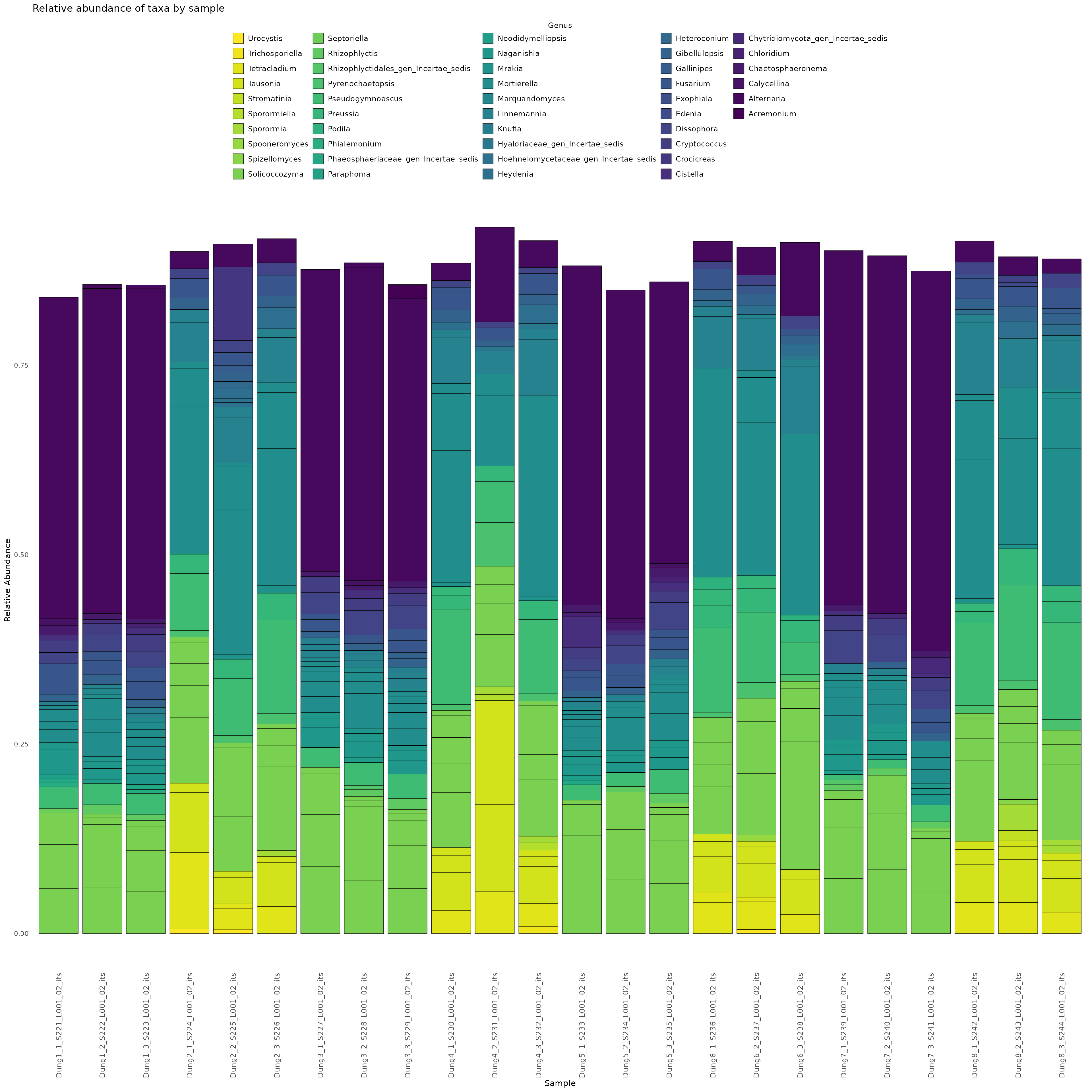
Here we demonstrate how to make a stacked bar plot of the relative abundance of taxa by sample for the ITS-barcoded samples
data <- objs$phyloseq_its %>%
  phyloseq::transform_sample_counts(function(x) {x/sum(x)} ) %>%
  phyloseq::psmelt() %>%
  dplyr::filter(Abundance > 0.005) %>%
  dplyr::arrange(Genus)

abund_plot <- ggplot2::ggplot(data, ggplot2::aes(x = Sample, y = Abundance, fill = Genus)) +
  ggplot2::geom_bar(stat = "identity", position = "stack", color = "black", size = 0.2) +
  ggplot2::scale_fill_viridis_d() +
  ggplot2::theme_minimal() +
  ggplot2::labs(
    y = "Relative Abundance",
    title = "Relative abundance of taxa by sample",
    fill = "Genus"
  ) +
  ggplot2::theme(
    axis.text.x = ggplot2::element_text(angle = 90, hjust = 1, vjust = 0.5, size = 10),
    panel.grid.major = ggplot2::element_blank(),
    panel.grid.minor = ggplot2::element_blank(),
    legend.position = "top",
    legend.text = ggplot2::element_text(size = 10),
    legend.title = ggplot2::element_text(size = 10),  # Adjust legend title size
    strip.text = ggplot2::element_text(size = 10),
    strip.background = ggplot2::element_blank()
  ) +
  ggplot2::guides(
    fill = ggplot2::guide_legend(
      reverse = TRUE,
      keywidth = 1,
      keyheight = 1,
      title.position = "top",
      title.hjust = 0.5,  # Center the legend title
      label.theme = ggplot2::element_text(size = 10)  # Adjust the size of the legend labels
    )
  )

print(abund_plot)
Finally,we demonstrate how to make a stacked bar plot of the relative abundance of taxa by sample for the rps10-barcoded samples
data <- objs$phyloseq_rps10 %>%
  phyloseq::transform_sample_counts(function(x) {x/sum(x)} ) %>%
  phyloseq::psmelt() %>%
  dplyr::filter(Abundance > 0.0005) %>%
  dplyr::arrange(Genus)

abund_plot <- ggplot2::ggplot(data, ggplot2::aes(x = Sample, y = Abundance, fill = Genus)) +
  ggplot2::geom_bar(stat = "identity", position = "stack", color = "black", size = 0.2) +
  ggplot2::scale_fill_viridis_d() +
  ggplot2::theme_minimal() +
  ggplot2::labs(
    y = "Relative Abundance",
    title = "Relative abundance of taxa by sample",
    fill = "Genus"
  ) +
  ggplot2::theme(
    axis.text.x = ggplot2::element_text(angle = 90, hjust = 1, vjust = 0.5, size = 10),
    panel.grid.major = ggplot2::element_blank(),
    panel.grid.minor = ggplot2::element_blank(),
    legend.position = "top",
    legend.text = ggplot2::element_text(size = 10),
    legend.title = ggplot2::element_text(size = 10),  # Adjust legend title size
    strip.text = ggplot2::element_text(size = 10),
    strip.background = ggplot2::element_blank()
  ) +
  ggplot2::guides(
    fill = ggplot2::guide_legend(
      reverse = TRUE,
      keywidth = 1,
      keyheight = 1,
      title.position = "top",
      title.hjust = 0.5,  # Center the legend title
      label.theme = ggplot2::element_text(size = 10)  # Adjust the size of the legend labels
    )
  )

print(abund_plot)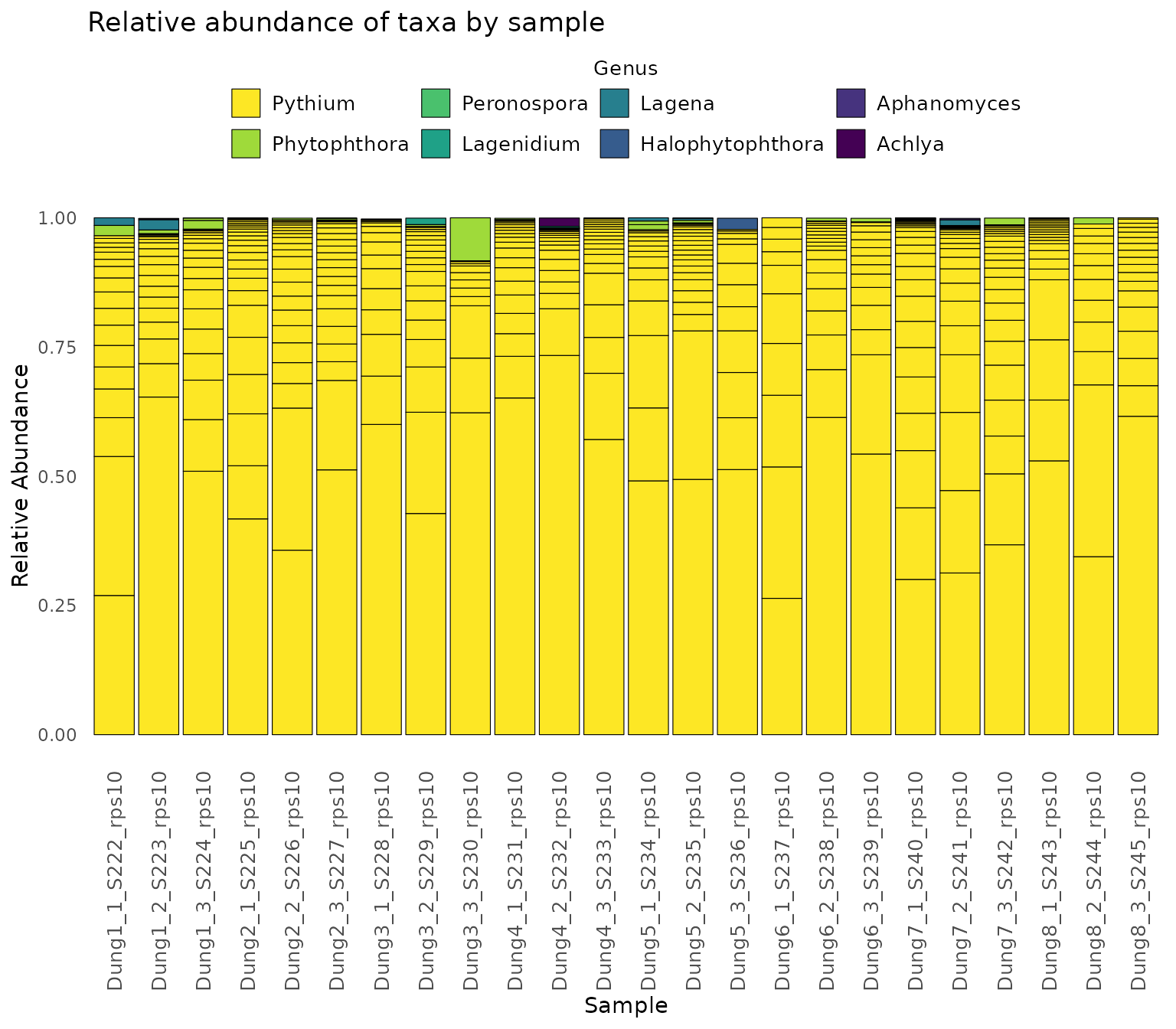
sessioninfo::session_info()
#> ─ Session info ───────────────────────────────────────────────────────────────
#>  setting  value
#>  version  R version 4.1.2 (2021-11-01)
#>  os       Pop!_OS 22.04 LTS
#>  system   x86_64, linux-gnu
#>  ui       X11
#>  language en
#>  collate  en_US.UTF-8
#>  ctype    en_US.UTF-8
#>  tz       America/Los_Angeles
#>  date     2024-07-29
#>  pandoc   3.1.1 @ /usr/lib/rstudio/resources/app/bin/quarto/bin/tools/ (via rmarkdown)
#>
#> ─ Packages ───────────────────────────────────────────────────────────────────
#>  ! package              * version    date (UTC) lib source
#>    ade4                   1.7-22     2023-02-06 [2] CRAN (R 4.1.2)
#>    ape                    5.8        2024-04-11 [2] CRAN (R 4.1.2)
#>    Biobase                2.54.0     2021-10-26 [2] Bioconductor
#>    BiocGenerics           0.40.0     2021-10-26 [2] Bioconductor
#>    BiocParallel           1.28.3     2021-12-09 [2] Bioconductor
#>    biomformat             1.22.0     2021-10-26 [2] Bioconductor
#>    Biostrings             2.62.0     2021-10-26 [2] Bioconductor
#>    bit                    4.0.5      2022-11-15 [2] CRAN (R 4.1.2)
#>    bit64                  4.0.5      2020-08-30 [4] CRAN (R 4.0.2)
#>    bitops                 1.0-7      2021-04-24 [4] CRAN (R 4.1.1)
#>    bslib                  0.7.0      2024-03-29 [2] CRAN (R 4.1.2)
#>    cachem                 1.1.0      2024-05-16 [2] CRAN (R 4.1.2)
#>    cli                    3.6.3      2024-06-21 [2] CRAN (R 4.1.2)
#>    cluster                2.1.2      2021-04-17 [5] CRAN (R 4.1.1)
#>    codetools              0.2-18     2020-11-04 [5] CRAN (R 4.0.3)
#>    colorspace             2.1-0      2023-01-23 [2] CRAN (R 4.1.2)
#>    crayon                 1.5.3      2024-06-20 [2] CRAN (R 4.1.2)
#>    dada2                  1.30.0     2024-01-20 [2] bioc_xgit (@ec87892)
#>    data.table             1.15.4     2024-03-30 [2] CRAN (R 4.1.2)
#>    DBI                    1.2.2      2024-02-16 [2] CRAN (R 4.1.2)
#>    DelayedArray           0.20.0     2021-10-26 [2] Bioconductor
#>    deldir                 2.0-4      2024-02-28 [2] CRAN (R 4.1.2)
#>  P demulticoder         * 0.0.0.9000 2024-07-29 [?] load_all()
#>    desc                   1.4.3      2023-12-10 [2] CRAN (R 4.1.2)
#>    devtools               2.4.3      2021-11-30 [4] CRAN (R 4.1.2)
#>    digest                 0.6.36     2024-06-23 [2] CRAN (R 4.1.2)
#>    dplyr                  1.1.4      2023-11-17 [2] CRAN (R 4.1.2)
#>    ellipsis               0.3.2      2021-04-29 [2] CRAN (R 4.1.2)
#>    evaluate               0.24.0     2024-06-10 [2] CRAN (R 4.1.2)
#>    fansi                  1.0.6      2023-12-08 [2] CRAN (R 4.1.2)
#>    farver                 2.1.2      2024-05-13 [2] CRAN (R 4.1.2)
#>    fastmap                1.2.0      2024-05-15 [2] CRAN (R 4.1.2)
#>    foreach                1.5.2      2022-02-02 [4] CRAN (R 4.1.2)
#>    fs                     1.6.4      2024-04-25 [2] CRAN (R 4.1.2)
#>    furrr                  0.3.1      2022-08-15 [2] CRAN (R 4.1.2)
#>    future                 1.33.2     2024-03-26 [2] CRAN (R 4.1.2)
#>    generics               0.1.3      2022-07-05 [2] CRAN (R 4.1.2)
#>    GenomeInfoDb           1.30.1     2022-01-30 [2] Bioconductor
#>    GenomeInfoDbData       1.2.7      2024-01-20 [2] Bioconductor
#>    GenomicAlignments      1.30.0     2021-10-26 [2] Bioconductor
#>    GenomicRanges          1.46.1     2021-11-18 [2] Bioconductor
#>    ggplot2                3.5.1      2024-04-23 [2] CRAN (R 4.1.2)
#>    globals                0.16.3     2024-03-08 [2] CRAN (R 4.1.2)
#>    glue                   1.7.0      2024-01-09 [2] CRAN (R 4.1.2)
#>    gtable                 0.3.5      2024-04-22 [2] CRAN (R 4.1.2)
#>    highr                  0.11       2024-05-26 [2] CRAN (R 4.1.2)
#>    hms                    1.1.3      2023-03-21 [2] CRAN (R 4.1.2)
#>    htmltools              0.5.8.1    2024-04-04 [2] CRAN (R 4.1.2)
#>    hwriter                1.3.2.1    2022-04-08 [2] CRAN (R 4.1.2)
#>    igraph                 2.0.3      2024-03-13 [2] CRAN (R 4.1.2)
#>    interp                 1.1-6      2024-01-26 [2] CRAN (R 4.1.2)
#>    IRanges                2.28.0     2021-10-26 [2] Bioconductor
#>    iterators              1.0.14     2022-02-05 [4] CRAN (R 4.1.2)
#>    jpeg                   0.1-10     2022-11-29 [2] CRAN (R 4.1.2)
#>    jquerylib              0.1.4      2021-04-26 [2] CRAN (R 4.1.2)
#>    jsonlite               1.8.8      2023-12-04 [2] CRAN (R 4.1.2)
#>    knitr                  1.48       2024-07-07 [2] CRAN (R 4.1.2)
#>    labeling               0.4.3      2023-08-29 [2] CRAN (R 4.1.2)
#>    lattice                0.20-45    2021-09-22 [5] CRAN (R 4.1.1)
#>    latticeExtra           0.6-30     2022-07-04 [2] CRAN (R 4.1.2)
#>    lazyeval               0.2.2      2019-03-15 [4] CRAN (R 4.0.1)
#>    lifecycle              1.0.4      2023-11-07 [2] CRAN (R 4.1.2)
#>    listenv                0.9.1      2024-01-29 [2] CRAN (R 4.1.2)
#>    magrittr               2.0.3      2022-03-30 [2] CRAN (R 4.1.2)
#>    MASS                   7.3-55     2022-01-13 [5] CRAN (R 4.1.2)
#>    Matrix                 1.4-0      2021-12-08 [5] CRAN (R 4.1.2)
#>    MatrixGenerics         1.6.0      2021-10-26 [2] Bioconductor
#>    matrixStats            1.2.0      2023-12-11 [2] CRAN (R 4.1.2)
#>    memoise                2.0.1      2021-11-26 [2] CRAN (R 4.1.2)
#>    metacoder              0.3.7      2024-02-20 [2] CRAN (R 4.1.2)
#>    mgcv                   1.8-39     2022-02-24 [5] CRAN (R 4.1.2)
#>    multtest               2.50.0     2021-10-26 [2] Bioconductor
#>    munsell                0.5.1      2024-04-01 [2] CRAN (R 4.1.2)
#>    nlme                   3.1-155    2022-01-13 [5] CRAN (R 4.1.2)
#>    parallelly             1.37.1     2024-02-29 [2] CRAN (R 4.1.2)
#>    permute                0.9-7      2022-01-27 [2] CRAN (R 4.1.2)
#>    phyloseq               1.46.0     2024-01-20 [2] bioc_xgit (@7320133)
#>    pillar                 1.9.0      2023-03-22 [2] CRAN (R 4.1.2)
#>    pkgbuild               1.4.4      2024-03-17 [2] CRAN (R 4.1.2)
#>    pkgconfig              2.0.3      2019-09-22 [2] CRAN (R 4.1.2)
#>    pkgdown                2.0.7      2022-12-14 [2] CRAN (R 4.1.2)
#>    pkgload                1.3.4      2024-01-16 [2] CRAN (R 4.1.2)
#>    plyr                   1.8.9      2023-10-02 [2] CRAN (R 4.1.2)
#>    png                    0.1-8      2022-11-29 [2] CRAN (R 4.1.2)
#>    purrr                * 1.0.2      2023-08-10 [2] CRAN (R 4.1.2)
#>    R6                     2.5.1      2021-08-19 [2] CRAN (R 4.1.2)
#>    ragg                   1.2.1      2021-12-06 [4] CRAN (R 4.1.2)
#>    RColorBrewer           1.1-3      2022-04-03 [2] CRAN (R 4.1.2)
#>    Rcpp                   1.0.13     2024-07-17 [2] CRAN (R 4.1.2)
#>    RcppParallel           5.1.7      2023-02-27 [2] CRAN (R 4.1.2)
#>    RCurl                  1.98-1.16  2024-07-11 [2] CRAN (R 4.1.2)
#>    readr                  2.1.5      2024-01-10 [2] CRAN (R 4.1.2)
#>    remotes                2.5.0      2024-03-17 [2] CRAN (R 4.1.2)
#>    reshape2               1.4.4      2020-04-09 [4] CRAN (R 4.0.1)
#>    rhdf5                  2.38.1     2022-03-10 [2] Bioconductor
#>    rhdf5filters           1.6.0      2021-10-26 [2] Bioconductor
#>    Rhdf5lib               1.16.0     2021-10-26 [2] Bioconductor
#>    rlang                  1.1.4      2024-06-04 [2] CRAN (R 4.1.2)
#>    rmarkdown              2.27       2024-05-17 [2] CRAN (R 4.1.2)
#>    rprojroot              2.0.4      2023-11-05 [2] CRAN (R 4.1.2)
#>    Rsamtools              2.10.0     2021-10-26 [2] Bioconductor
#>    rstudioapi             0.16.0     2024-03-24 [2] CRAN (R 4.1.2)
#>    S4Vectors              0.32.4     2022-03-24 [2] Bioconductor
#>    sass                   0.4.9      2024-03-15 [2] CRAN (R 4.1.2)
#>    scales                 1.3.0      2023-11-28 [2] CRAN (R 4.1.2)
#>    sessioninfo            1.2.2      2021-12-06 [2] CRAN (R 4.1.2)
#>    ShortRead              1.60.0     2024-01-20 [2] bioc_xgit (@4304db4)
#>    stringi                1.8.4      2024-05-06 [2] CRAN (R 4.1.2)
#>    stringr                1.5.1      2023-11-14 [2] CRAN (R 4.1.2)
#>    SummarizedExperiment   1.24.0     2021-10-26 [2] Bioconductor
#>    survival               3.2-13     2021-08-24 [5] CRAN (R 4.1.1)
#>    systemfonts            1.0.4      2022-02-11 [4] CRAN (R 4.1.2)
#>    textshaping            0.3.6      2021-10-13 [4] CRAN (R 4.1.1)
#>    tibble                 3.2.1      2023-03-20 [2] CRAN (R 4.1.2)
#>    tidyr                  1.3.1      2024-01-24 [2] CRAN (R 4.1.2)
#>    tidyselect             1.2.1      2024-03-11 [2] CRAN (R 4.1.2)
#>    tzdb                   0.4.0      2023-05-12 [2] CRAN (R 4.1.2)
#>    usethis                2.1.5      2021-12-09 [4] CRAN (R 4.1.2)
#>    utf8                   1.2.4      2023-10-22 [2] CRAN (R 4.1.2)
#>    vctrs                  0.6.5      2023-12-01 [2] CRAN (R 4.1.2)
#>    vegan                  2.6-6.1    2024-05-21 [2] CRAN (R 4.1.2)
#>    viridisLite            0.4.2      2023-05-02 [2] CRAN (R 4.1.2)
#>    vroom                  1.6.5      2023-12-05 [2] CRAN (R 4.1.2)
#>    withr                  3.0.0      2024-01-16 [2] CRAN (R 4.1.2)
#>    xfun                   0.46       2024-07-18 [2] CRAN (R 4.1.2)
#>    XVector                0.34.0     2021-10-26 [2] Bioconductor
#>    yaml                   2.3.9      2024-07-05 [2] CRAN (R 4.1.2)
#>    zlibbioc               1.40.0     2021-10-26 [2] Bioconductor
#>
#>  [1] /tmp/Rtmpni2SLp/temp_libpath2824e9279530a5
#>  [2] /home/marthasudermann/R/x86_64-pc-linux-gnu-library/4.1
#>  [3] /usr/local/lib/R/site-library
#>  [4] /usr/lib/R/site-library
#>  [5] /usr/lib/R/library
#>
#>  P ── Loaded and on-disk path mismatch.
#>
#> ──────────────────────────────────────────────────────────────────────────────