Reading VCF data
BJ Knaus, JF Tabima and NJ Grünwald
Genetic variation data is typically stored in variant call format (VCF) files (Danecek et al., 2011). This format is the preferred file format obtained from genome sequencing or high throughput genotyping. One advantage of using VCF files is that only variants (e.g., SNPs, indels, etc.) are reported which economizes files size relative to a format that may included invariant sites. Variant callers typically attempt to aggressively call variants with the perspective that a downstream quality control step will remove low quality variants. Note that VCF files come in different flavors and that each variant caller may report a slightly different information. A first step in working with this data is to understand their contents.
VCF file structure
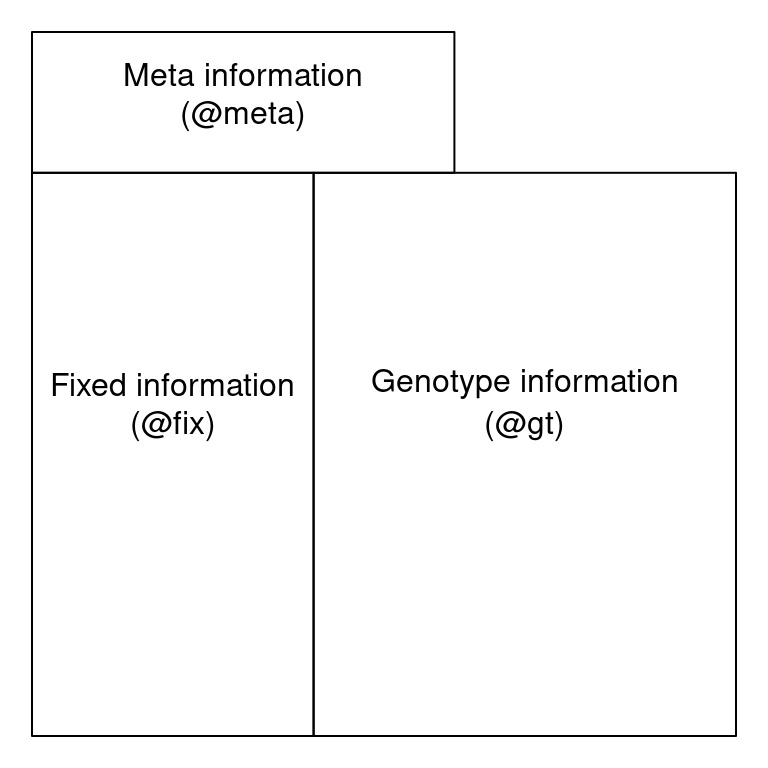
A VCF file can be thought of as having three sections: a vcf header, a fix region and a gt region. The VCF meta region is located at the top of the file and contains meta-data describing the body of the file. Each VCF meta line begins with a ‘##’. The information in the meta region defines the abbreviations used elsewhere in the file. It may also document software used to create the file as well as parameters used by this software. Below the metadata region, the data are tabular. The first eight columns of this table contain information about each variant. This data may be common over all variants, such as its chromosomal position, or a summary over all samples, such as quality metrics. These data are fixed, or the same, over all samples. The fix region is required in a VCF file, subsequent columns are optional but are common in our experience. Beginning at column ten is a column for every sample. The values in these columns are information for each sample and each variant. The organization of each cell containing a genotype and associated information is specified in column nine, the FORMAT column. The location of these three regions within a file can be represented by this cartoon:

Cartoon representation of VCF file organization
The VCF file specification is flexible. This means that there are slots for certain types of data, but any particular software which creates a VCF file does not necessarily use them all. Similarly, authors have the opportunity to include new forms of data, forms which may not have been foreseen by the authors of the VCF specification. The result is that all VCF files do not contain the same information.
For this example, we will use example data provided with the R package vcfR (Knaus & Grünwald, 2017).
## ***** Object of Class vcfR *****
## 18 samples
## 1 CHROMs
## 2,533 variants
## Object size: 3.2 Mb
## 8.497 percent missing data
## *****        *****         *****
The function library() loads libraries, in this case the package vcfR. The function data() loads datasets that were included with R and its packages. Our usage of data() loads the objects ‘gff’, ‘dna’ and ‘vcf’ from the ‘vcfR_example’ dataset. Here we’re only interested in the object ‘vcf’ which contains example VCF data. When we call the object name with no function it invokes the ‘show’ method which prints some summary information to the console.
The meta region
The meta region contains information about the file, its creation, as well as information to interpret abbreviations used elsewhere in the file. Each line of the meta region begins with a double pound sign (‘##’). The example which comes with vcfR is shown below. (Only the first seven lines are shown for brevity.)
## [1] "##fileformat=VCFv4.1"
## [2] "##source=\"GATK haplotype Caller, phased with beagle4\""
## [3] "##FILTER=<ID=LowQual,Description=\"Low quality\">"
## [4] "##FORMAT=<ID=AD,Number=.,Type=Integer,Description=\"Allelic depths for the ref and alt alleles in the order listed\">"
## [5] "##FORMAT=<ID=DP,Number=1,Type=Integer,Description=\"Approximate read depth (reads with MQ=255 or with bad mates are filtered)\">"
## [6] "##FORMAT=<ID=GQ,Number=1,Type=Integer,Description=\"Genotype Quality\">"
## [7] "##FORMAT=<ID=GT,Number=1,Type=String,Description=\"Genotype\">"
The first line contains the version of the VCF format used in the file. This line is required. The second line specifies the software which created the VCF file. This is not required, so not all VCF files include it. When they do, the file becomes self documenting. Note that the alignment software is not included here because it was used upstream of the VCF file’s creation (aligners typically create *.SAM or *.BAM format files). Because the file can only include information about the software that created it, the entire pipeline does not get documented. Some VCF files may contain a line for every chromosome (or supercontig or contig depending on your genome), so they may become rather long. Here, the remaining lines contain INFO and FORMAT specifications which define abbreviations used in the fix and gt portions of the file.
The meta region may include long lines that may not be easy to view. In vcfR we’ve created a function to help press this data.
##  [1] "FILTER=ID=LowQual"                    "FORMAT=ID=AD"                         "FORMAT=ID=DP"                         "FORMAT=ID=GQ"                         "FORMAT=ID=GT"
##  [6] "FORMAT=ID=PL"                         "GATKCommandLine=ID=HaplotypeCaller"   "INFO=ID=AC"                           "INFO=ID=AF"                           "INFO=ID=AN"
## [11] "INFO=ID=BaseQRankSum"                 "INFO=ID=ClippingRankSum"              "INFO=ID=DP"                           "INFO=ID=DS"                           "INFO=ID=FS"
## [16] "INFO=ID=HaplotypeScore"               "INFO=ID=InbreedingCoeff"              "INFO=ID=MLEAC"                        "INFO=ID=MLEAF"                        "INFO=ID=MQ"
## [21] "INFO=ID=MQ0"                          "INFO=ID=MQRankSum"                    "INFO=ID=QD"                           "INFO=ID=ReadPosRankSum"               "INFO=ID=SOR"
## [26] "1 contig=<IDs omitted from queryMETA"
When the function queryMETA() is called with only a vcfR object as a parameter, it attempts to summarize the meta information. Not all of the information is returned. For example, ‘contig’ elements are not returned. This is an attempt to summarize information that may be most useful for comprehension of the file’s contents.
## [[1]]
## [1] "FORMAT=ID=DP"                                                                          "Number=1"
## [3] "Type=Integer"                                                                          "Description=Approximate read depth (reads with MQ=255 or with bad mates are filtered)"
##
## [[2]]
## [1] "INFO=ID=DP"                                                            "Number=1"
## [3] "Type=Integer"                                                          "Description=Approximate read depth; some reads may have been filtered"
When an element parameter is included, only the information about that element is returned. In this example the element ‘DP’ is returned. We see that this acronym is defined as both a ‘FORMAT’ and ‘INFO’ acronym. We can narrow down our query by including more information in the element parameter.
## [[1]]
## [1] "FORMAT=ID=DP"                                                                          "Number=1"
## [3] "Type=Integer"                                                                          "Description=Approximate read depth (reads with MQ=255 or with bad mates are filtered)"
Here we’ve isolated the definition of ‘DP’ as a ‘FORMAT’ element. Note that the function queryMETA() includes the parameter nice which by default is TRUE and attempts to present the data in a nicely formatted manner. However, our query is performed on the actual information in the ‘meta’ region. It is therefore sometimes appropriate to set nice = FALSE so that we can see the raw data. In the above example the angled bracket (‘<’) is omitted from the nice = TRUE representation but is essential to distinguishing the ‘FORMAT’ element from the ‘INFO’ element.
The fix region
The fix region contains information for each variant which is sometimes summarized over all samples. The first eight columns of the fixed region are titled CHROM, POS, ID, REF, ALT, QUAL, FILTER and INFO. This is per variant information which is ‘fixed’, or the same, over all samples. The first two columns indicate the location of the variant by chromosome and position within that chromosome. Here, the ID field has not been used, so it consists of missing data (NA). The REF and ALT columns indicate the reference and alternate allelic states for a diploid sample. When multiple alternate allelic states are present they are delimited with commas. The QUAL column attempts to summarize the quality of each variant over all samples. The FILTER field is not used here but could contain information on whether a variant has passed some form of quality assessment.
##      CHROM              POS   ID REF ALT QUAL     FILTER
## [1,] "Supercontig_1.50" "2"   NA "T" "A" "44.44"  NA
## [2,] "Supercontig_1.50" "246" NA "C" "G" "144.21" NA
## [3,] "Supercontig_1.50" "549" NA "A" "C" "68.49"  NA
## [4,] "Supercontig_1.50" "668" NA "G" "C" "108.07" NA
## [5,] "Supercontig_1.50" "765" NA "A" "C" "92.78"  NA
## [6,] "Supercontig_1.50" "780" NA "G" "T" "58.38"  NA
The eigth column, titled INFO, is a semicolon delimited list of information. It can be rather long and cumbersome. The function getFIX() will suppress this column by default. Each abbreviation in the INFO column should be defined in the meta section. We can validate this by querying the meta portion, as we did in the ‘meta’ section above.
The gt region
The gt (genotype) region contains information about each variant for each sample. The values for each variant and each sample are colon delimited. Multiple types of data for each genotype may be stored in this manner. The format of the data is specified by the FORMAT column (column nine). Here we see that we have information for GT, AD, DP, GQ and PL. The definition of these acronyms can be referenced by querying the the meta region, as demonstrated previously. Every variant does not necessarily have the same information (e.g., SNPs and indels may be handled differently), so the rows are best treated independently. Different variant callers may include different information in this region.
##      FORMAT           BL2009P4_us23               DDR7602                   IN2009T1_us22
## [1,] "GT:AD:DP:GQ:PL" "0|0:62,0:62:99:0,190,2835" "0|0:12,0:12:39:0,39,585" "0|0:37,0:37:99:0,114,1709"
## [2,] "GT:AD:DP:GQ:PL" "1|0:5,5:10:99:111,0,114"   NA                        "0|1:2,1:3:16:16,0,48"
## [3,] "GT:AD:DP:GQ:PL" NA                          NA                        "0|0:2,0:2:6:0,6,51"
## [4,] "GT:AD:DP:GQ:PL" "0|0:1,0:1:3:0,3,44"        NA                        "1|1:0,1:1:3:25,3,0"
## [5,] "GT:AD:DP:GQ:PL" "0|0:2,0:2:6:0,6,49"        "0|0:1,0:1:3:0,3,34"      "0|0:1,0:1:3:0,3,31"
## [6,] "GT:AD:DP:GQ:PL" "0|0:2,0:2:6:0,6,49"        "0|0:1,0:1:3:0,3,34"      "0|0:3,0:3:9:0,9,85"
vcfR
Using the R package vcfR, we can read VCF format files into memory using the function read.vcfR(). Once in memory we can use the head() method to summarize the information in the three VCF regions.
## Scanning file to determine attributes.
## File attributes:
##   meta lines: 29
##   header_line: 30
##   variant count: 2190
##   column count: 27
##
Meta line 29 read in.
## All meta lines processed.
## gt matrix initialized.
## Character matrix gt created.
##   Character matrix gt rows: 2190
##   Character matrix gt cols: 27
##   skip: 0
##   nrows: 2190
##   row_num: 0
##
Processed variant 1000
Processed variant 2000
Processed variant: 2190
## All variants processed
## [1] "***** Object of class 'vcfR' *****"
## [1] "***** Meta section *****"
## [1] "##fileformat=VCFv4.1"
## [1] "##source=\"GATK haplotype Caller, phased with beagle4\""
## [1] "##FILTER=<ID=LowQual,Description=\"Low quality\">"
## [1] "##FORMAT=<ID=AD,Number=.,Type=Integer,Description=\"Allelic depths fo [Truncated]"
## [1] "##FORMAT=<ID=DP,Number=1,Type=Integer,Description=\"Approximate read  [Truncated]"
## [1] "##FORMAT=<ID=GQ,Number=1,Type=Integer,Description=\"Genotype Quality\">"
## [1] "First 6 rows."
## [1]
## [1] "***** Fixed section *****"
##      CHROM              POS     ID REF ALT       QUAL      FILTER
## [1,] "Supercontig_1.50" "80058" NA "T" "G,TACTG" "3480.23" NA
## [2,] "Supercontig_1.50" "80063" NA "C" "T"       "3016.89" NA
## [3,] "Supercontig_1.50" "80067" NA "A" "C"       "3555.08" NA
## [4,] "Supercontig_1.50" "80073" NA "C" "A"       "104.72"  NA
## [5,] "Supercontig_1.50" "80074" NA "A" "G"       "2877.74" NA
## [6,] "Supercontig_1.50" "80089" NA "A" "ACG"     "2250.92" NA
## [1]
## [1] "***** Genotype section *****"
##      FORMAT           BL2009P4_us23                              DDR7602                                   IN2009T1_us22                               LBUS5
## [1,] "GT:AD:DP:GQ:PL" "1|0:25,3,0:28:45:45,0,1120,129,1134,1300" "1|0:19,7,0:26:99:237,0,777,300,804,1181" "0|1:29,6,0:35:99:162,0,1229,252,1252,1512" "0|1:19,7,0:26:99:237,0,777,300,804,1181"
## [2,] "GT:AD:DP:GQ:PL" "1|0:29,3:32:30:30,0,1335"                 "1|0:20,7:27:99:234,0,819"                "0|1:27,7:34:99:204,0,1232"                 "0|1:20,7:27:99:234,0,819"
## [3,] "GT:AD:DP:GQ:PL" "1|0:31,3:34:27:27,0,1372"                 "1|0:19,6:25:99:189,0,864"                "0|1:27,6:33:99:210,0,1155"                 "0|1:19,6:25:99:189,0,864"
## [4,] "GT:AD:DP:GQ:PL" "0|0:30,0:30:99:0,102,1530"                "0|0:26,0:26:87:0,87,1305"                "0|0:33,0:33:99:0,99,1485"                  "0|0:26,0:26:87:0,87,1305"
## [5,] "GT:AD:DP:GQ:PL" "0|0:30,0:30:93:0,93,1395"                 "1|0:21,4:25:99:147,0,867"                "0|1:27,6:33:99:171,0,1116"                 "0|1:21,4:25:99:147,0,867"
## [6,] "GT:AD:DP:GQ:PL" "0|0:33,0:33:99:0,99,1485"                 "1|0:20,2:22:18:18,0,918"                 "0|1:27,7:34:99:213,0,1113"                 "0|1:20,2:22:18:18,0,918"
##      NL07434
## [1,] "0|1:45,19,0:64:99:643,0,1782,793,1866,2825"
## [2,] "0|1:42,18:60:99:655,0,1748"
## [3,] "0|1:41,16:57:99:584,0,1737"
## [4,] "0|0:56,0:56:99:0,172,2565"
## [5,] "0|1:39,16:55:99:629,0,1709"
## [6,] "0|1:34,12:46:99:393,0,1518"
## [1] "First 6 columns only."
## [1]
## [1] "Unique GT formats:"
## [1] "GT:AD:DP:GQ:PL"
## [1]
After we have made any manipulations of the file we can save it as a VCF file with the function write.vcf().
write.vcf()will write a file to your active directory. We now have a summary of our VCF file which we can use to help understand what forms of information are contained within it. This information can be further explored with plotting functions and used to filter the VCF file for high quality variants as we will see in the next section.
Exercises
1) How would we find more information about read.vcfR()?
2) How would we learn what the acronym “AD” stands for?
3) We used the head() function to view the first few lines of fix data. How would we view the last few lines of fix data?
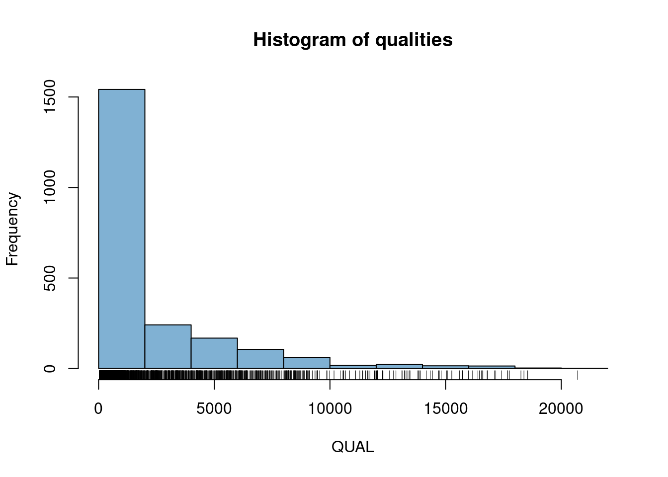
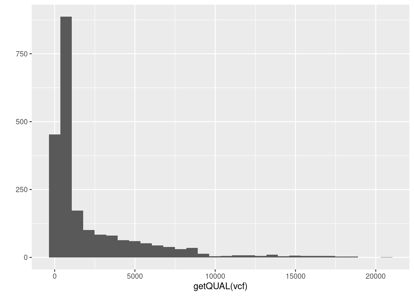
4) There is a column in the fix portion of the data called QUAL. It is not defined in the meta portion of the data because it is defined in the VCF specification. It stands for ‘quality’. Does QUAL appear useful to us? Why or why not?
5) How would we query the sample names?
Note that the first column is FORMAT. This tells us the format for data for each variant. According to the VCF specification this can be different for each variant.
References
Danecek P., Auton A., Abecasis G., Albers CA., Banks E., DePristo MA., Handsaker RE., Lunter G., Marth GT., Sherry ST. et al. 2011. The variant call format and VCFtools. Bioinformatics 27:2156–2158. Available at: https://doi.org/10.1093/bioinformatics/btr330
Knaus BJ., Grünwald NJ. 2017. \({V}cfr\): A package to manipulate and visualize variant call format data in R. Molecular Ecology Resources 17:44–53. Available at: http://dx.doi.org/10.1111/1755-0998.12549

