Introduction to R
This appendix introduces basic use of the R statistical and computer language and the RStudio Desktop integrated development environment (IDE). We assume you installed the needed resources mentioned in chapter 2 on getting ready to use R.
Warning: To install R and RStudio you might need administrator privileges. Contact your IT manager and ask for an R installation or administrator privileges.
After installing both R and RStudio, please proceed to open RStudio. RStudio should look something like:
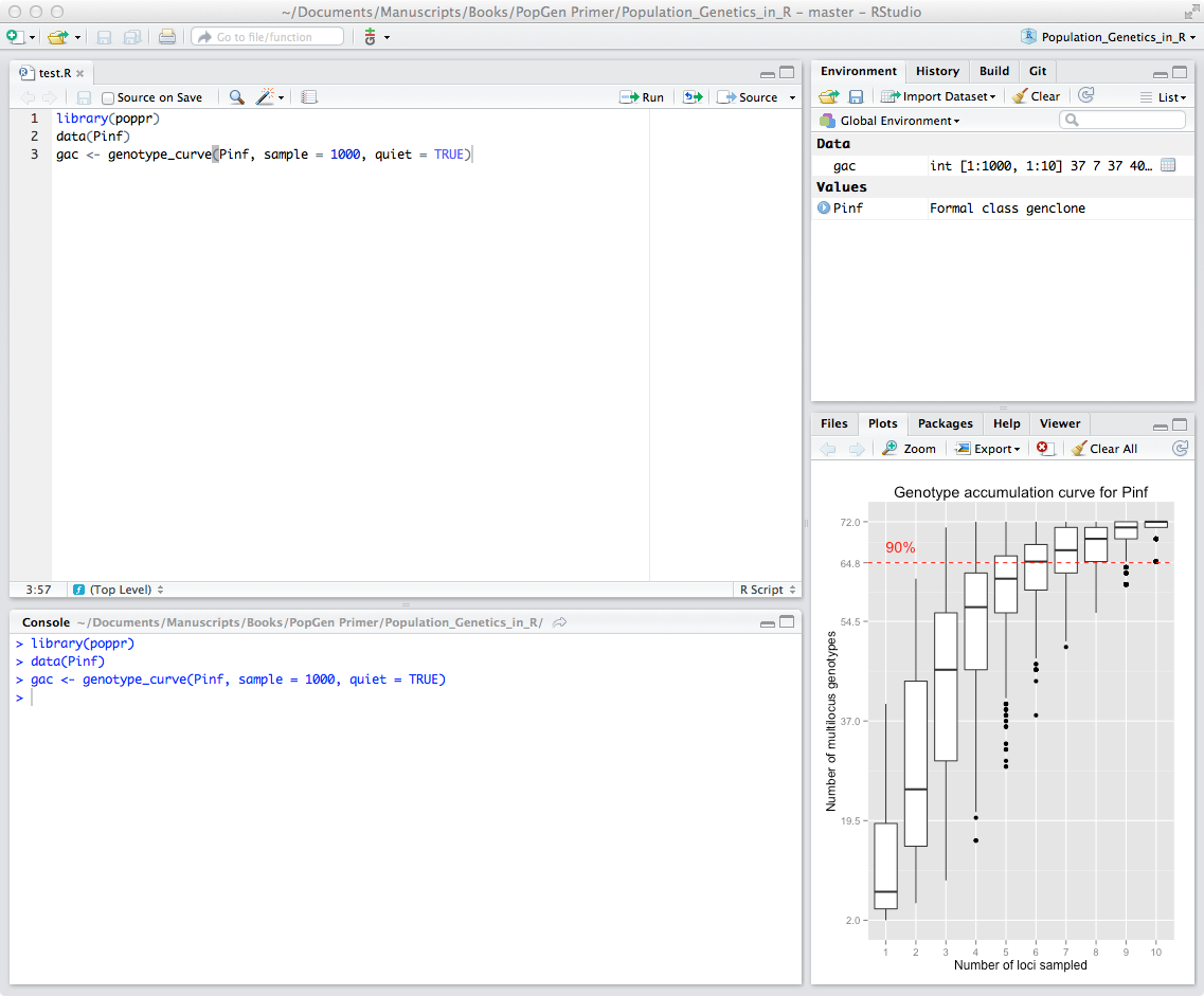
RStudio
The top left panel is a text-box where you can write a script. The bottom left panel is the console (or command line) where you directly execute commands and R writes results to the console; for example, type in x <- 1 hit return and then type x and hit return again and watch the console:
Note: the “>” symbol is R’s prompt for you to type something in the console.
[1] 1You just assigned the value 1 to the variable x with the assignment operator <-. The second command asks R to show the value assigned to R. Finally, the top right panel shows variables loaded into the environment and the bottom right panel is useful for loading files, plotting graphs, installing packages and getting help. Feel free to explore all the various tabs or elements of each panel.
Assignment, data types and operations
Let’s learn a few simple facts about R:
R uses # to add comments to code:
[1] 2This is very useful when developing reusable code or when you want to remember a few months later what you actually did.
R is case sensitive so that x <- 5 is not the same as X <- x + 1. Try typing this into your console and look at x and X, respectively:
[1] 5[1] 6Next, let’s assign numbers to a vector:
[1] 1 2 3 4 5You can see several important traits of R. The c() command (which stands for combine) can be used to make a list (e.g., a vector) of data. We can overwrite the variable x with new content and we can assign another data type (e.g., a single number becomes a vector). To compound things further you can even change the data type to strings overwriting the previous content:
[1] "Paris" "Tokyo" "Seattle"Note that we use quotes to denote the string data type containing text.
To access individual elements of a vector, in this case the second element, we execute:
[1] "Tokyo"Creating RStudio projects
Coding projects usually results in a vast number of files, datasets, scripts and figures that can be difficult to manage and keep organized. RStudio has created the RStudio projects to facilitate and simplify the management a project by associating all of the project files into a working directory of your preference. This means that all script files, datasets and results of a project can be stored in a set location to facilitate access and management.
To create and RStudio project, we need to go to the upper right corner of RStudio, and click on New Project:
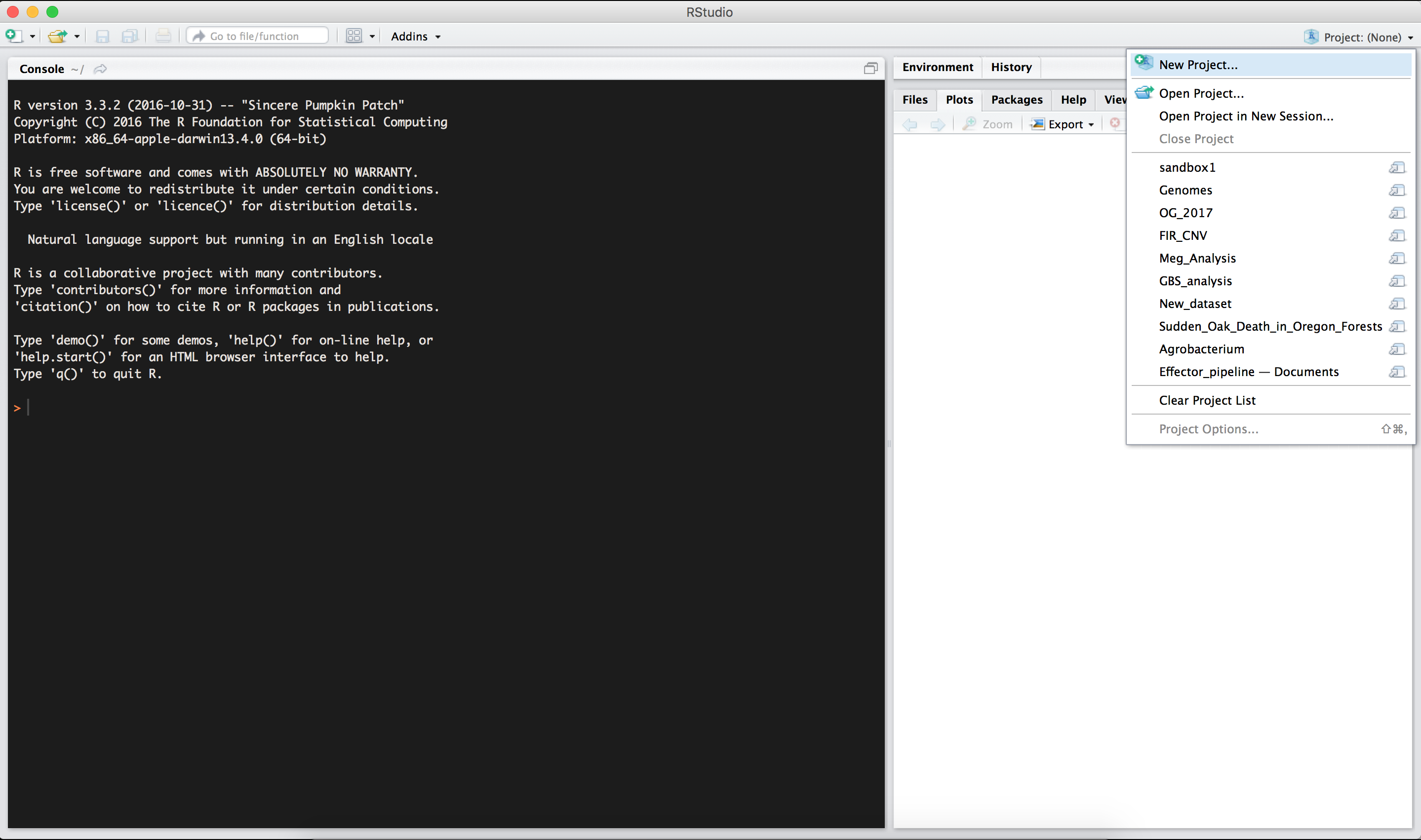
A pop-up window should appear. We want to create a new directory in our desktop to store our data and keep our files. To create the directory click on New Directory:
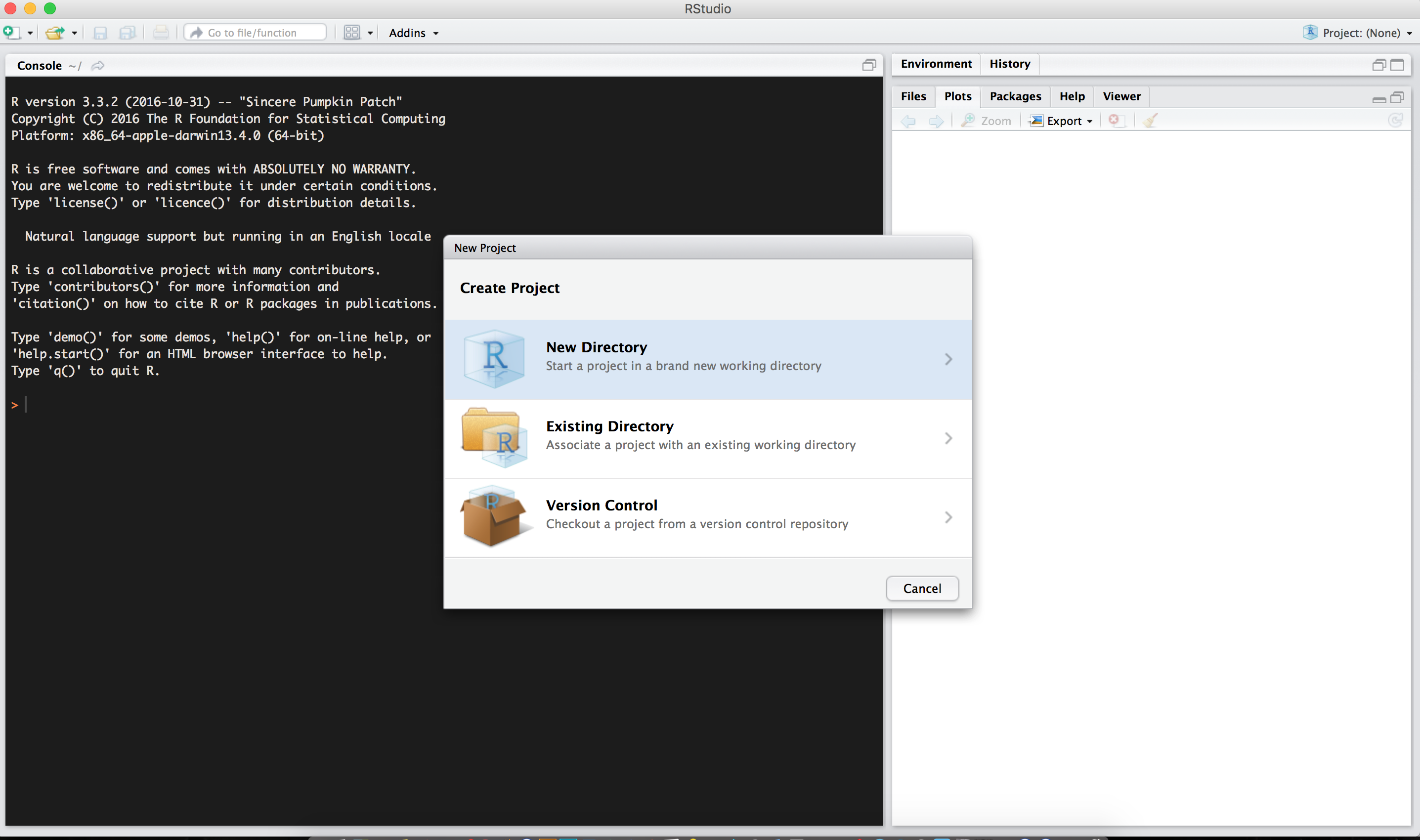
Since we are starting this project from scratch, we will select the Empty Project option. This will create a new RStudio project:
Then, we will use APS_Workshop as the name for our new directory, and we will create the directory as a subdirectory of your desktop:
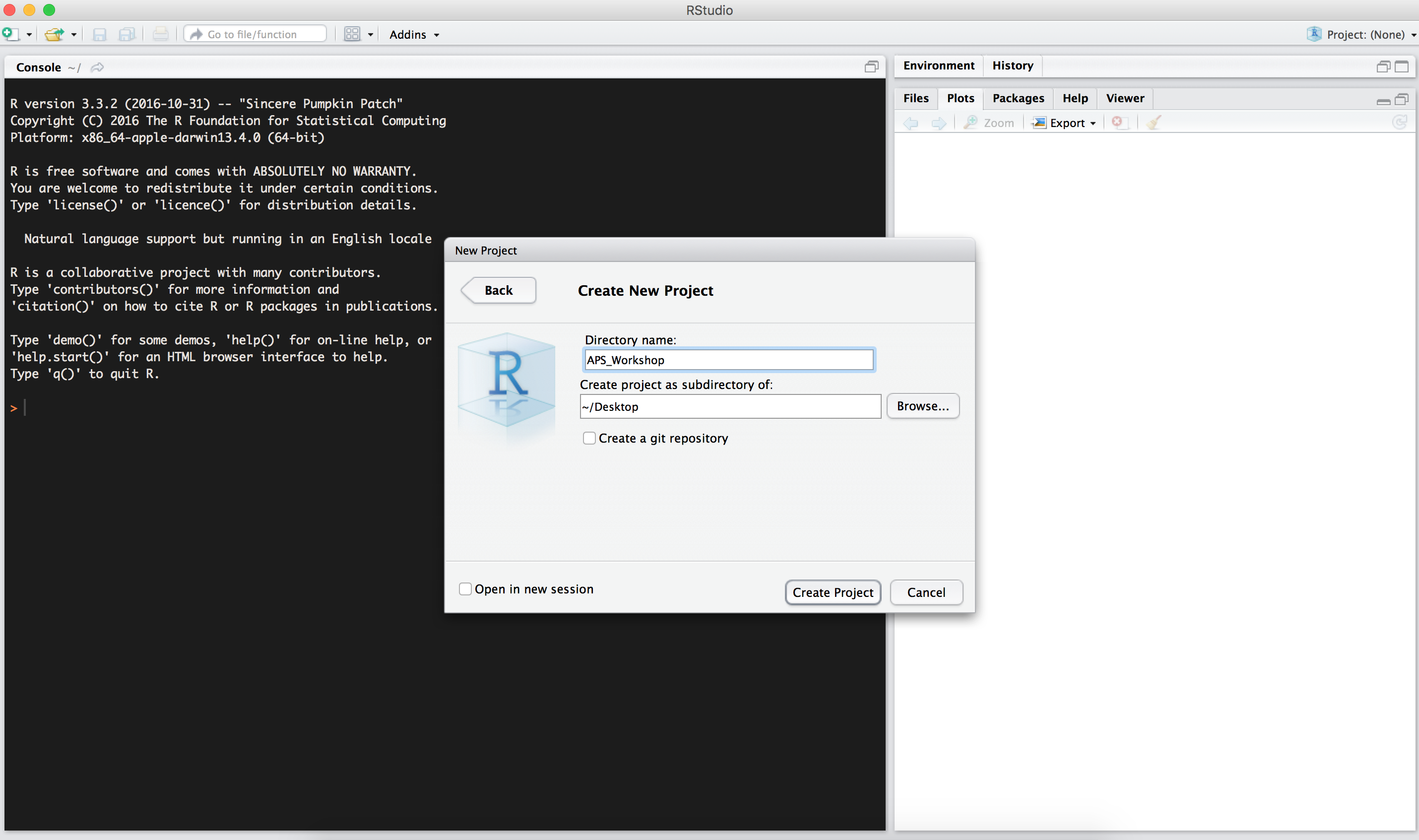
And there is your new RStudio project withing the APS_Workshop directory! We can start downloading the required files and scripts for the workshop into that folder.
Console tricks: Code completion & command history
RStudio has a very useful feature called code completion using the Tab key which can complete the full name of an object. For example type hel and hit Tab and you will see several functions pop up and you can select help().
This also works inside a function to find function arguments. Type help( and hit Tab to select arguments for the help function.
RStudio records your command history. Thus you can scroll up or down the history of executed commands using the Up or Down arrows. Make sure your cursor is in the console and try to re-execute previous commands.
To quit R you can either use the RStudio > Quit pull-down menu command or execute ⌘ + Q (OS X) or ctrl + Q (PC).
Getting help
One way that R shines above other languages for analysis is the fact that R packages in CRAN are all documented. Help files are written in HTML and give the user a brief overview of:
- The purpose of a function
- The parameters it takes
- The output it yields
- Some examples demonstrating its usage.
To see all of the help topics in a package, you can simply type:
help(package = "poppr") # Get help for a package.
help(amova)             # Get help for the amova function.
?amova                  # same as above.
??multilocus            # Search for functions that have the keyword multilocus.
Some packages include vignettes that can have different formats such as being introductions, tutorials, or reference cards in PDF format. You can look at a list of vignettes in all packages by typing:
browseVignettes()                  # see vignettes from all packages
browseVignettes(package = 'poppr') # see vignettes from a specific package.
and to look at a specific vignette you can type:
Useful resources to learn R
Introductory
- Swirl is a very well thought out R package that teaches you interactively.
- Code School Try R is a nice interactive tutorial.
- Quick R
- R reference card
- A very nice, short introduction to R
Advanced
- Advanced R by Hadley Wickham
Books:
- R in a Nutshell
- R cookbook is a nice quick reference and tutorial for general R use.
- ggplot2 book is a useful reference if you want to customize graphs for publication.