Before starting, first take a look at the Quickstart for instructions on how to download pathogensurveillance and install both Docker and Nextflow.
Example 1: Standard Run
This example uses sequencing reads from an 2022 outbreak of the bacterial pathogen Xanthomonas hortorum found infecting geranium in several plant nurseries. Using whole-genome sequencing, researchers determined a shared genetic basis between strains at different locations. With this information, they traced the origin of the outbreak to a single supplier that sold infected cuttings. You can read more about the study here.
We’ll be treating the pathogen as an unknown and using the pathogensurveillance pipeline to determine what we know already (that these samples come from Xanthomonas hortorum). We’ll also see the high degree of shared DNA sequence between samples, which is seen from several plots that the pathogensurveillance pipeline generates automatically.
Sample input
The pipeline is designed to work with a wide variety of existing metadata sheets without extensive changes. Here’s a look at “xanthomonas.csv”, which serves as the only unique input file within the command to run the pipeline:
Warning: package 'tidyverse' was built under R version 4.1.2
Warning: package 'tibble' was built under R version 4.1.2
Warning: package 'forcats' was built under R version 4.1.2
sample_id
path_1
path_2
sequence_type
reference
reference_id
report_group
color_by
date_isolated
date_received
year
host
cv_key
nursery
X
X.1
22-299
test/data/reads/22-299_R1.fastq.gz
test/data/reads/22-299_R2.fastq.gz
Illumina
xan_test
subgroup
year
nursery
3/2/22
3/29/22
2022
Pelargonium x hortorum
CV-1
MD
22-300
test/data/reads/22-300_R1.fastq.gz
test/data/reads/22-300_R2.fastq.gz
Illumina
xan_test
subgroup
year
nursery
3/2/22
3/30/22
2022
Pelargonium x hortorum
CV-2
MD
22-301
test/data/reads/22-301_R1.fastq.gz
test/data/reads/22-301_R2.fastq.gz
Illumina
xan_test
subgroup
year
nursery
3/2/22
3/31/22
2022
Pelargonium x hortorum
CV-3
MD
22-302
test/data/reads/22-302_R1.fastq.gz
test/data/reads/22-302_R2.fastq.gz
Illumina
xan_test
subgroup
year
nursery
3/2/22
4/1/22
2022
Pelargonium x hortorum
CV-4
MD
22-303
test/data/reads/22-303_R1.fastq.gz
test/data/reads/22-303_R2.fastq.gz
Illumina
xan_test
subgroup
year
nursery
3/2/22
4/2/22
2022
Pelargonium x hortorum
CV-5
MD
22-304
test/data/reads/22-304_R1.fastq.gz
test/data/reads/22-304_R2.fastq.gz
Illumina
xan_test
subgroup
year
nursery
3/7/22
4/3/22
2022
Pelargonium x hortorum
CV-6
MD
There is quite a bit of information in this file, but only a few columns are essential (and can be in any order). The input csv needs show the pipeline where to find the sequencing reads. These can either be present locally or they can be downloaded from the NCBI.
Sample ID: The “sample_id” column is used to name your samples. This information will be used in graphs, so it is recommended to keep names short but informative. If you do not include this column, sample IDs will be generated from the names of your fastq files.
Using local reads: Columns “path_1” and “path_2” specify the path to forward and reverse reads. Each row corresponds to one individual sample. Reads for this tutorial are hosted on the pathogensurveilance github repo. . If your reads are single-ended, “path_2” should be left blank.
Shortread/Longread sequences*: Information in the column “sequencing_type” tells the pipeline these are derived from illumina shortreads. Other options for this column are “nanopore” and “pacbio”.
Downloading reads: Sequence files may instead be hosted on the NCBI. In that case, the “shortread_1/shortread_2” columns should be substituted with a single “SRA” column, and they will be downloaded right after the pipeline checks the sample sheet. These downloads will show up in the folder path_surveil_data/reads. See test/data/metadata/xanthomonas.csv for an example using this input format.
Specifying a reference genome (optional): The “reference_refseq” column may be useful when you are relatively confident as to the identity of your samples and would like to include one particular reference for comparison. See Example 2 for an explanation of how to designate mandatory and optional references.
Assigning sample groups (optional): The optional column “color_by” is used for data visualization. It will assign one or more columns to serve as grouping factors for the output report. Here, samples will be grouped by the values of the “year” and “nursery” columns. Note that multiple factors need to be separated by semicolons within the color_by column.
Running the pipeline
Here is the full command used execute this example, using a docker container:
When running your own analysis, you will need to provide your own path to the input CSV file.
By default, the pipeline will run on 128 GB of RAM and 16 threads. These are more resources than are strictly necessary and beyond the capacity of most desktop computers. We can scale this back a bit for this lightweight test run. This analysis will work with 8 CPUs and 30 GB of RAM (albeit more slowly), which is specified by the –max_cpus and –max_memory settings.
The setting -resume is only necessary when resuming a previous analysis. However, it doesn’t hurt to include it at the start. If the pipeline is interrupted, this setting allows progress to pick up where it left off – as long as the previous command is executed from the same working directory.
If the pipeline begins successfully, you should see a screen tracking your progress:
[25/63dcee] process > PATHOGENSURVEILLANCE:INPUT_CHECK:SAMPLESHEET_CHECK (xanthomonas.csv)[100%] 1 of 1[- ] process > PATHOGENSURVEILLANCE:SRATOOLS_FASTERQDUMP -[- ] process > PATHOGENSURVEILLANCE:DOWNLOAD_ASSEMBLIES -[- ] process > PATHOGENSURVEILLANCE:SEQKIT_SLIDING -[- ] process > PATHOGENSURVEILLANCE:FASTQC -[- ] process > PATHOGENSURVEILLANCE:COARSE_SAMPLE_TAXONOMY:BBMAP_SENDSKETCH -
The input and output of each process can be accessed from the work/ directory. The subdirectory within work/ is designated by the string to left of each step. Note that this location will be different each time the pipeline is run, and only the first part of the name of the subdirectory is shown. For this run, we could navigate to work/25/63dcee(etc) to access the input csv that is used for the next step.
Report
You should see a message similar to this if the pipeline finishes successfully:
-[nf-core/plantpathsurveil] Pipeline completed successfully-To clean the cache, enter the command: nextflow clean evil_boyd -fCompleted at: 20-May-2024 12:44:40Duration : 3h 29m 2sCPU hours : 15.2Succeeded : 253
The final report can be viewed as either a .pdf or .html file. It can be accessed inside the reports folder of the output directory (here: xanthomonas/reports). This report shows several key pieces of information about your samples.
A note on storage management - pathogensurveillance creates a large number of intermediate files. For most users we recommend clearing these files after each run. To do so, run the script shown after the completion message (nextflow clean -f). You would not want to do this if: (1) You still need to use the caching system. For example, imagine you would like to compare a new sample to 10 samples from a previous run. In that case, some files could be reused to make the pipeline work more quickly. (2) You would like to use intermediate files for your own analysis. By default, these files are saved in the output directory as symlinks to their location in the work/ directory, so you would need to retrieve these before clearing the cache. You could use alternatively use the option –copymode high to save all intermediate files to the published directory, though in the short term this doubles the storage footprint of each run.
This particular report has been included as an example
Summary:
Pipeline Status Report: error messages for samples or sample groups
Input Data: Data read from the input .csv file
Identification:
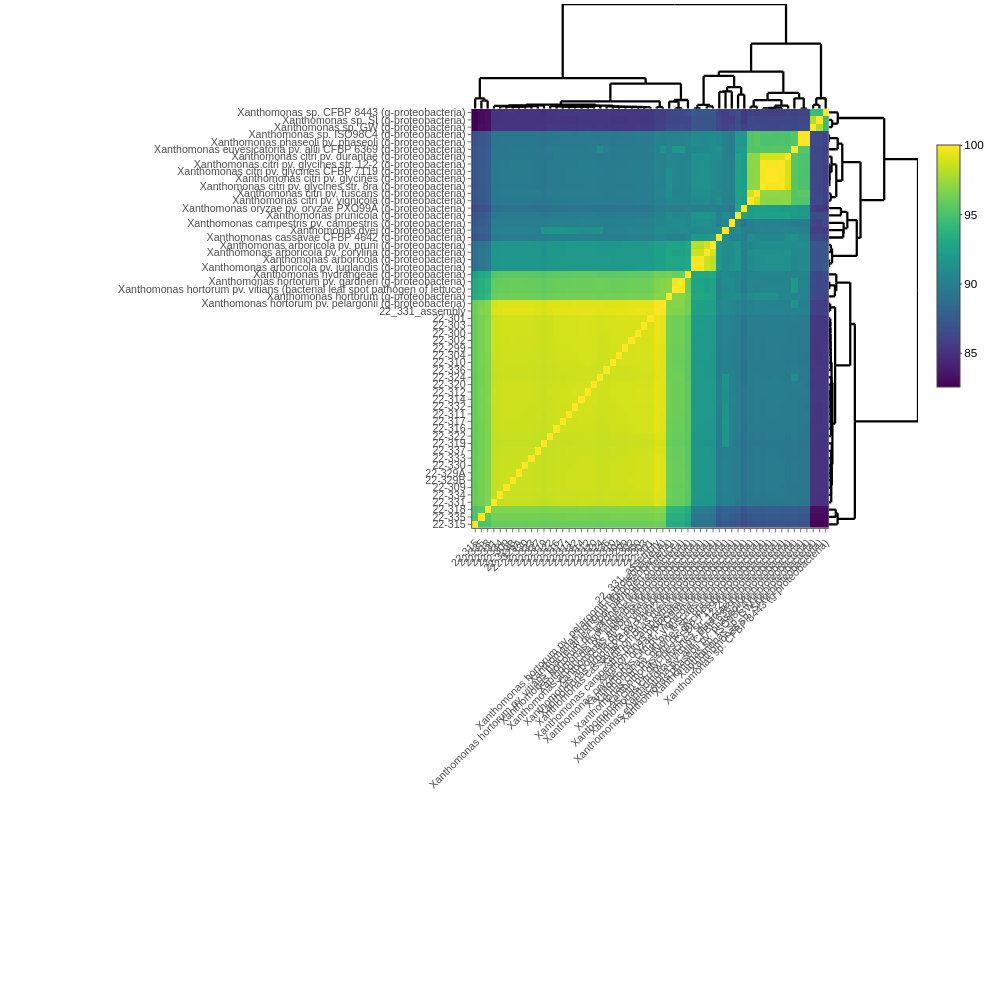
Initial identification: Coarse identification from the bbmap sendsketch step. The first tab shows best species ID for each sample. The second tab shows similarity metrics between sample sequences and other reference genomes: %ANI (average nucleotide identity), %WKID (weighted kmer identity), and %completeness.
For more information about each metric, click the About this table tab underneath.
Most similar organisms: Shows relationships between samples and references using % ani and % pocp (percentage of conserved proteins). For better resolution, you can interactively zoom in/out of plots.
Core gene phylogeny: A core gene phylogeny uses the sequences of all gene shared by all of the genomes included in the tree to infer evolutionary relationships. It is the most robust identification provided by this pipeline, but its precision is still limited by the availability of similar reference sequences. Methods to generate this tree differ between prokaryotes and eukaryotes. Our input to the pipeline was prokaryotic DNA sequences, and the method to build this tree is based upon many different core genes shared between samples and references (for eukaryotes, this is constrained to BUSCO genes). This tree is built with iqtree and based upon shared core genes analyzed using the program pirate.
SNP trees: This tree is better suited for visualizing the genetic diversity among samples. However, the core gene phylogeny provides a much better source of information for evolutionary differences among samples and other known references.
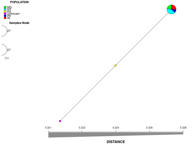
Minimum spanning network
Minimum spanning network: The nodes represent unique multilocus genotypes, and the size of nodes is proportional to the # number of samples that share the same genotype. The edges represent the SNP differences between two given genotypes, and the darker the color of the edges, the fewer SNP differences between the two.
Example 2: Defining References
If you know what your samples are already, you may want to tell the pipeline to use a “standard” reference genome instead of picking one that is more obscure – even if pathogensurveillance deems the alternative to be a better fit. Other users may have a few different organisms of interest that they want to use as a points of comparison. For example, maybe there is a particularly nasty strain of V. cholerae that you want to see in relation to your other samples. There are a few options to select (or not select) reference genomes for these cases.
Pathogensurveillance uses two categories of reference genomes. Primary references are used for alignment and will always be displayed in phylogenetic trees. In contrast, contextual references are selected before the primary reference is known and they may or may not be used later. Some contextual references are chosen because they are really close matches to your samples, and these may be selected to become primary references. However, pathogensurveillance will select a few distantly related contextual references too. Some of these are used to “fill out” the phylogeny, and you may want a higher or lower number of contextual references depending on how you want your phylogenetic trees to look.
Chosing primary references
Take this sample list containing three Mycobacterium abscessus samples and three Mycobacterium leprae samples:
sample_id
ncbi.accession
mycobacterium_abscessus1
ERR7253671
mycobacterium_abscessus2
ERR7253669
mycobacterium_abscessus3
ERR7253671
mycobacterium_leperae1
SRR6241707
mycobacterium_leperae2
SRR6241708
mycobacterium_leperae3
SRR6241709
To force the pipeline to use the NCBI specified Mycobacterium abscessus reference genome for the three Mycobacterium abscessus samples, and likewise make the three Mycobacterium leprae samples use the NCBI specified Mycobacterium leprae genome, we need to tell pathogensurveillance both where to find these reference sequences and how to use them. We can either specify a local path to the reads, or this can instead be specified through the ref_ncbi_accession column. Here, how the references are used here is controlled by the ref_primary_usage column:
sample_id
ncbi.accession
ref_ncbi_accession
ref_primary_usage
mycobacterium_abscessus1
ERR7253671
GCF_001632805.1
required
mycobacterium_abscessus2
ERR7253669
GCF_001632805.1
required
mycobacterium_abscessus3
ERR7253671
GCF_001632805.1
required
mycobacterium_leprae1
SRR6241707
GCF_003253775.1
required
mycobacterium_leprae2
SRR6241708
GCF_003253775.1
required
mycobacterium_leprae3
SRR6241709
GCF_003253775.1
required
Specifying contextual references
Taking the previous Mycobacterium abscessus/leprae example, imagine we would like to see the comparison between Mycobacterium abscessus and Mycobacterium tuberculosis. We can do this by including Mycobacterium tuberculosis as a mandatory contextual reference:
sample_id
ncbi.accession
ref_ncbi_accession
ref_contextual_usage
mycobacterium_abscessus1
ERR7253671
GCF_001632805.1
required
mycobacterium_abscessus2
ERR7253669
GCF_001632805.1
required
mycobacterium_abscessus3
ERR7253671
GCF_001632805.1
required
mycobacterium_leprae1
SRR6241707
mycobacterium_leprae2
SRR6241708
mycobacterium_leprae3
SRR6241709
Selecting references from an NCBI query
It is also possible to submit a valid NCBI query to the pipeline with reference genomes selected from query hits. For example, you could test how your Mycobacterium leprae samples compared to a bunch of different other Mycobacterium leprae genomes:
sample_id
ncbi.accession
ref_ncbi_query
ref_ncbi_query_max
mycobacterium_abscessus1
ERR7253671
NA
mycobacterium_abscessus2
ERR7253669
NA
mycobacterium_abscessus3
ERR7253671
NA
mycobacterium_leprae1
SRR6241707
mycobacterium leprae
100
mycobacterium_leprae2
SRR6241708
mycobacterium leprae
100
mycobacterium_leprae3
SRR6241709
mycobacterium leprae
100
Some things to keep in mind:
Depending on your organism, this may a massive amount of data. Make sure you have queried NCBI beforehand to get a good handle on how many references you are downloading.
The optional parameter ref_ncbi_query_max is a good way of limiting this number when you are sampling from a densely populated clade, such as Mycobacterium leprae. This parameter can either be a set number (like shown here) or a percentage.
The NCBI API will fail if there are too many requests. See ncbi support for more detail.
Multiple references per sample
If we would like to add multiple references per sample, we can enter this information through a separate reference csv. In this example, we specify one primary reference each for Mycobacterium abscessus and Mycobacterium leprae, then three additional contextual references for Mycobacterium leprae: