Perform Analysis of Molecular Variance (AMOVA) on genind or genclone objects.

This function simplifies the process necessary for performing AMOVA in R. It gives user the choice of utilizing either the ade4 or the pegas implementation of AMOVA. See ade4::amova() (ade4) and pegas::amova() (pegas) for details on the specific implementation.

Usage

poppr.amova(
  x,
  hier = NULL,
  clonecorrect = FALSE,
  within = TRUE,
  dist = NULL,
  squared = TRUE,
  freq = TRUE,
  correction = "quasieuclid",
  sep = "_",
  filter = FALSE,
  threshold = 0,
  algorithm = "farthest_neighbor",
  threads = 1L,
  missing = "loci",
  cutoff = 0.05,
  quiet = FALSE,
  method = c("ade4", "pegas"),
  nperm = 0
)

Arguments

x

a genind, genclone, genlight, or snpclone object

hier

a hierarchical formula that defines your population hierarchy. (e.g.: ~Population/Subpopulation). See Details below.

clonecorrect

logical if TRUE, the data set will be clone corrected with respect to the lowest level of the hierarchy. The default is set to FALSE. See clonecorrect() for details.

within

logical. When this is set to TRUE (Default), variance within individuals are calculated as well. If this is set to FALSE, The lowest level of the hierarchy will be the sample level. See Details below.

dist

an optional distance matrix calculated on your data. If this is set to NULL (default), the raw pairwise distances will be calculated via dist().

squared

if a distance matrix is supplied, this indicates whether or not it represents squared distances.

freq

logical. If within = FALSE, the parameter rho is calculated (Ronfort et al. 1998; Meirmans and Liu 2018). By setting freq = TRUE, (default) allele counts will be converted to frequencies before the distance is calculated, otherwise, the distance will be calculated on allele counts, which can bias results in mixed-ploidy data sets. Note that this option has no effect for haploid or presence/absence data sets.

correction

a character defining the correction method for non-euclidean distances. Options are ade4::quasieuclid() (Default), ade4::lingoes(), and ade4::cailliez(). See Details below.

sep

Deprecated. As of poppr version 2, this argument serves no purpose.

filter

logical When set to TRUE, mlg.filter will be run to determine genotypes from the distance matrix. It defaults to FALSE. You can set the parameters with algorithm and threshold arguments. Note that this will not be performed when within = TRUE. Note that the threshold should be the number of allowable substitutions if you don't supply a distance matrix.

threshold

a number indicating the minimum distance two MLGs must be separated by to be considered different. Defaults to 0, which will reflect the original (naive) MLG definition.

algorithm

determines the type of clustering to be done.

"farthest_neighbor": (default) merges clusters based on the maximum distance between points in either cluster. This is the strictest of the three.
"nearest_neighbor": merges clusters based on the minimum distance between points in either cluster. This is the loosest of the three.
"average_neighbor": merges clusters based on the average distance between every pair of points between clusters.

threads

integer When using filtering or genlight objects, this parameter specifies the number of parallel processes passed to mlg.filter() and/or bitwise.dist().

missing

specify method of correcting for missing data utilizing options given in the function missingno(). Default is "loci". This only applies to genind or genclone objects.

cutoff

specify the level at which missing data should be removed/modified. See missingno() for details. This only applies to genind or genclone objects.

quiet

logical If FALSE (Default), messages regarding any corrections will be printed to the screen. If TRUE, no messages will be printed.

method

Which method for calculating AMOVA should be used? Choices refer to package implementations: "ade4" (default) or "pegas". See details for differences.

nperm

the number of permutations passed to the pegas implementation of amova.

Value

a list of class amova from the ade4 or pegas package. See ade4::amova() or pegas::amova() for details.

Details

The poppr implementation of AMOVA is a very detailed wrapper for the ade4 implementation. The output is an ade4::amova() class list that contains the results in the first four elements. The inputs are contained in the last three elements. The inputs required for the ade4 implementation are:

a distance matrix on all unique genotypes (haplotypes)
a data frame defining the hierarchy of the distance matrix
a genotype (haplotype) frequency table.

All of this data can be constructed from a genind or genlight object, but can be daunting for a novice R user. This function automates the entire process. Since there are many variables regarding genetic data, some points need to be highlighted:

On Hierarchies:

The hierarchy is defined by different population strata that separate your data hierarchically. These strata are defined in the strata slot of genind, genlight, genclone, and snpclone objects. They are useful for defining the population factor for your data. See the function strata() for details on how to properly define these strata.

On Within Individual Variance:

Heterozygosities within genotypes are sources of variation from within individuals and can be quantified in AMOVA. When within = TRUE, poppr will split genotypes into haplotypes with the function make_haplotypes() and use those to calculate within-individual variance. No estimation of phase is made. This acts much like the default settings for AMOVA in the Arlequin software package. Within individual variance will not be calculated for haploid individuals or dominant markers as the haplotypes cannot be split further. Setting within = FALSE uses the euclidean distance of the allele frequencies within each individual. Note: within = TRUE is incompatible with filter = TRUE. In this case, within will be set to FALSE

On Euclidean Distances:

With the ade4 implementation of AMOVA (utilized by poppr), distances must be Euclidean (due to the nature of the calculations). Unfortunately, many genetic distance measures are not always euclidean and must be corrected for before being analyzed. Poppr automates this with three methods implemented in ade4, quasieuclid(), lingoes(), and cailliez(). The correction of these distances should not adversely affect the outcome of the analysis.

On Filtering:

Filtering multilocus genotypes is performed by mlg.filter(). This can necessarily only be done AMOVA tests that do not account for within-individual variance. The distance matrix used to calculate the amova is derived from using mlg.filter() with the option stats = "distance", which reports the distance between multilocus genotype clusters. One useful way to utilize this feature is to correct for genotypes that have equivalent distance due to missing data. (See example below.)

On Methods:

Both ade4 and pegas have implementations of AMOVA, both of which are appropriately called "amova". The ade4 version is faster, but there have been questions raised as to the validity of the code utilized. The pegas version is slower, but careful measures have been implemented as to the accuracy of the method. It must be noted that there appears to be a bug regarding permuting analyses where within individual variance is accounted for (within = TRUE) in the pegas implementation. If you want to perform permutation analyses on the pegas implementation, you must set within = FALSE. In addition, while clone correction is implemented for both methods, filtering is only implemented for the ade4 version.

On Polyploids:

As of poppr version 2.7.0, this function is able to calculate phi statistics for within-individual variance for polyploid data with full dosage information. When a data set does not contain full dosage information for all samples, then the resulting pseudo-haplotypes will contain missing data, which would result in an incorrect estimate of variance.

Instead, the AMOVA will be performed on the distance matrix derived from allele counts or allele frequencies, depending on the freq option. This has been shown to be robust to estimates with mixed ploidy (Ronfort et al. 1998; Meirmans and Liu 2018). If you wish to brute-force your way to estimating AMOVA using missing values, you can split your haplotypes with the make_haplotypes() function.

One strategy for addressing ambiguous dosage in your polyploid data set would be to convert your data to polysat's genambig class with the as.genambig(), estimate allele frequencies with polysat::deSilvaFreq(), and use these frequencies to randomly sample alleles to fill in the ambiguous alleles.

References

Excoffier, L., Smouse, P.E. and Quattro, J.M. (1992) Analysis of molecular variance inferred from metric distances among DNA haplotypes: application to human mitochondrial DNA restriction data. Genetics, 131, 479-491.

Ronfort, J., Jenczewski, E., Bataillon, T., and Rousset, F. (1998). Analysis of population structure in autotetraploid species. Genetics, 150, 921–930.

Meirmans, P., Liu, S. (2018) Analysis of Molecular Variance (AMOVA) for Autopolyploids Submitted.

Examples

data(Aeut)
strata(Aeut) <- other(Aeut)$population_hierarchy[-1]
agc <- as.genclone(Aeut)
agc
#> 
#> This is a genclone object
#> -------------------------
#> Genotype information:
#> 
#>    119 original multilocus genotypes 
#>    187 diploid individuals
#>     56 dominant loci
#> 
#> Population information:
#> 
#>      2 strata - Pop, Subpop
#>      2 populations defined - Athena, Mt. Vernon
amova.result <- poppr.amova(agc, ~Pop/Subpop)
#> 
#>  No missing values detected.
amova.result
#> $call
#> ade4::amova(samples = xtab, distances = xdist, structures = xstruct)
#> 
#> $results
#>                             Df    Sum Sq     Mean Sq
#> Between Pop                  1 1051.2345 1051.234516
#> Between samples Within Pop  16  273.4575   17.091091
#> Within samples             169  576.5059    3.411277
#> Total                      186 1901.1979   10.221494
#> 
#> $componentsofcovariance
#>                                            Sigma          %
#> Variations  Between Pop                11.063446  70.006786
#> Variations  Between samples Within Pop  1.328667   8.407483
#> Variations  Within samples              3.411277  21.585732
#> Total variations                       15.803391 100.000000
#> 
#> $statphi
#>                         Phi
#> Phi-samples-total 0.7841427
#> Phi-samples-Pop   0.2803128
#> Phi-Pop-total     0.7000679
#> 
amova.test <- randtest(amova.result) # Test for significance
plot(amova.test)

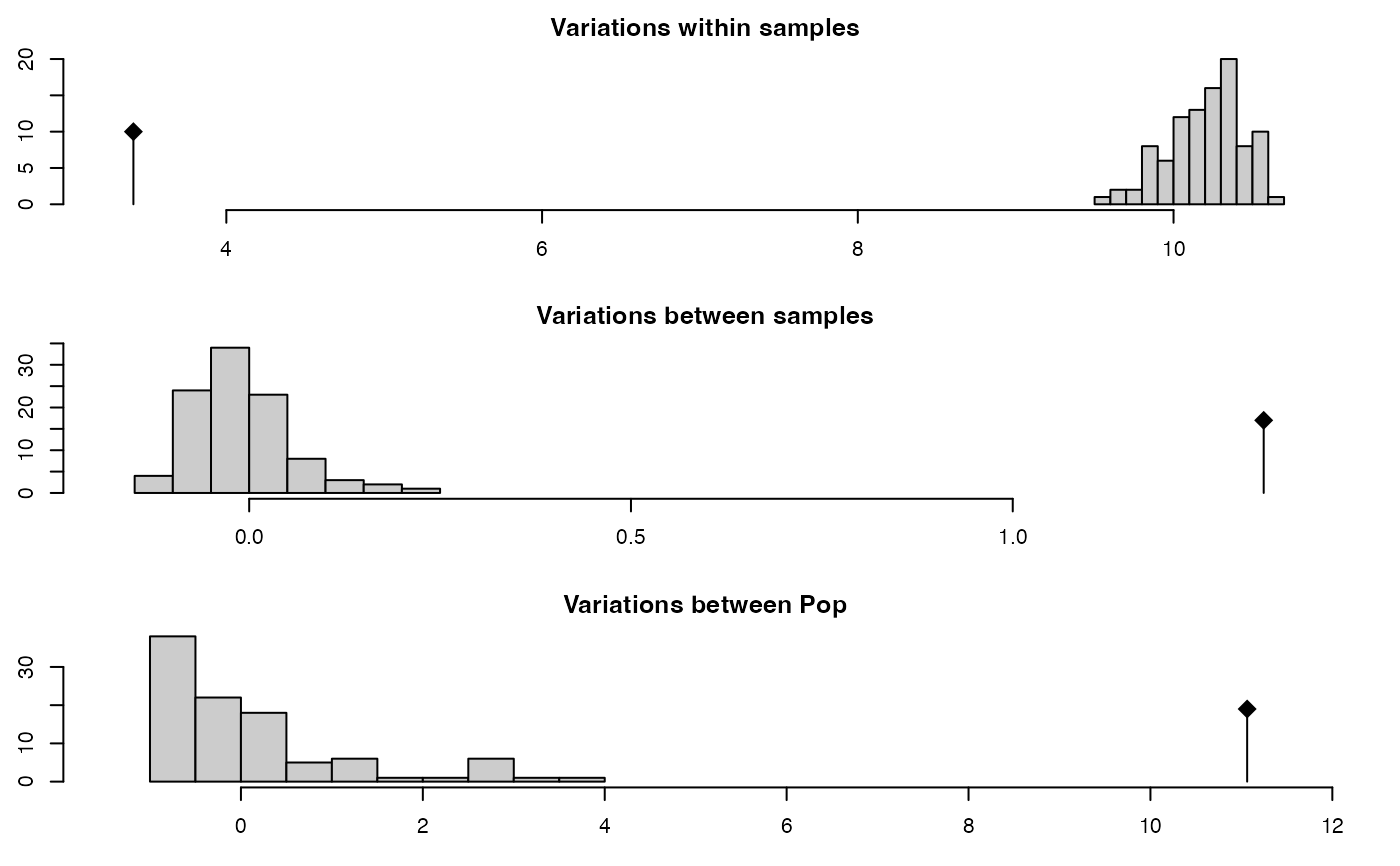amova.test
#> class: krandtest lightkrandtest 
#> Monte-Carlo tests
#> Call: randtest.amova(xtest = amova.result)
#> 
#> Number of tests:   3 
#> 
#> Adjustment method for multiple comparisons:   none 
#> Permutation number:   99 
#>                         Test       Obs   Std.Obs   Alter Pvalue
#> 1  Variations within samples  3.411277 -28.82359    less   0.01
#> 2 Variations between samples  1.328667  20.76983 greater   0.01
#> 3     Variations between Pop 11.063446  10.20109 greater   0.01
#> 

# \dontrun{

# You can get the same results with the pegas implementation
amova.pegas <- poppr.amova(agc, ~Pop/Subpop, method = "pegas")
#> 
#>  No missing values detected.
#> Warning: Zero distance(s)
amova.pegas
#> 
#> 	Analysis of Molecular Variance
#> 
#> Call: pegas::amova(formula = hier, data = hierdf, nperm = nperm, is.squared = FALSE)
#> 
#>              SSD         MSD  df
#> Pop    1051.2345 1051.234516   1
#> Subpop  273.4575   17.091091  16
#> Error   576.5059    3.411277 169
#> Total  1901.1979   10.221494 186
#> 
#> Variance components:
#>       Pop    Subpop     Error 
#> 11.063446  1.328667  3.411277 
#> 
#> Phi-statistics:
#>    Pop.in.GLOBAL (Phi_CT) Subpop.in.GLOBAL (Phi_ST)    Subpop.in.Pop (Phi_SC) 
#>                 0.7000679                 0.7841427                 0.2803128 
#> 
#> Variance coefficients:
#>        a        b        c 
#> 10.29589 11.16949 93.36898 
#> 
amova.pegas$varcomp/sum(amova.pegas$varcomp)
#>        Pop     Subpop      Error 
#> 0.70006786 0.08407483 0.21585732 

# Clone correction is possible
amova.cc.result <- poppr.amova(agc, ~Pop/Subpop, clonecorrect = TRUE)
#> 
#>  No missing values detected.
amova.cc.result
#> $call
#> ade4::amova(samples = xtab, distances = xdist, structures = xstruct)
#> 
#> $results
#>                             Df    Sum Sq    Mean Sq
#> Between Pop                  1  741.9872 741.987234
#> Between samples Within Pop  16  185.6877  11.605483
#> Within samples             123  520.1123   4.228555
#> Total                      140 1447.7872  10.341337
#> 
#> $componentsofcovariance
#>                                             Sigma          %
#> Variations  Between Pop                10.4131525  66.777680
#> Variations  Between samples Within Pop  0.9520545   6.105355
#> Variations  Within samples              4.2285550  27.116965
#> Total variations                       15.5937620 100.000000
#> 
#> $statphi
#>                         Phi
#> Phi-samples-total 0.7288303
#> Phi-samples-Pop   0.1837727
#> Phi-Pop-total     0.6677768
#> 
amova.cc.test <- randtest(amova.cc.result)
plot(amova.cc.test)

amova.cc.test
#> class: krandtest lightkrandtest 
#> Monte-Carlo tests
#> Call: randtest.amova(xtest = amova.cc.result)
#> 
#> Number of tests:   3 
#> 
#> Adjustment method for multiple comparisons:   none 
#> Permutation number:   99 
#>                         Test        Obs    Std.Obs   Alter Pvalue
#> 1  Variations within samples  4.2285550 -20.171106    less   0.01
#> 2 Variations between samples  0.9520545   9.802126 greater   0.01
#> 3     Variations between Pop 10.4131525   9.237767 greater   0.01
#> 


# Example with filtering
data(monpop)
splitStrata(monpop) <- ~Tree/Year/Symptom
poppr.amova(monpop, ~Symptom/Year) # gets a warning of zero distances
#> 
#>  No loci with missing values above 5% found.
#> Warning: Zero distance(s)
#> Distance matrix is non-euclidean.
#> Using quasieuclid correction method. See ?quasieuclid for details.
#> Warning: Zero distance(s)
#> $call
#> ade4::amova(samples = xtab, distances = xdist, structures = xstruct)
#> 
#> $results
#>                                 Df     Sum Sq    Mean Sq
#> Between Symptom                  1   17.62137  17.621372
#> Between samples Within Symptom   4  444.47746 111.119364
#> Within samples                 688 4880.09229   7.093157
#> Total                          693 5342.19112   7.708789
#> 
#> $componentsofcovariance
#>                                                 Sigma          %
#> Variations  Between Symptom                -0.3380505  -4.369677
#> Variations  Between samples Within Symptom  0.9811742  12.682763
#> Variations  Within samples                  7.0931574  91.686913
#> Total variations                            7.7362812 100.000000
#> 
#> $statphi
#>                             Phi
#> Phi-samples-total    0.08313087
#> Phi-samples-Symptom  0.12151770
#> Phi-Symptom-total   -0.04369677
#> 
poppr.amova(monpop, ~Symptom/Year, filter = TRUE, threshold = 0.1) # no warning
#> Filtering ...
#> Original multilocus genotypes   ... 264
#> Contracted multilocus genotypes ... 236
#> 
#>  No loci with missing values above 5% found.
#> Distance matrix is non-euclidean.
#> Using quasieuclid correction method. See ?quasieuclid for details.
#> $call
#> ade4::amova(samples = xtab, distances = xdist, structures = xstruct)
#> 
#> $results
#>                                 Df     Sum Sq    Mean Sq
#> Between Symptom                  1   18.13215  18.132145
#> Between samples Within Symptom   4  452.34660 113.086650
#> Within samples                 688 5002.62587   7.271259
#> Total                          693 5473.10462   7.897698
#> 
#> $componentsofcovariance
#>                                                 Sigma          %
#> Variations  Between Symptom                -0.3430635  -4.328197
#> Variations  Between samples Within Symptom  0.9980498  12.591711
#> Variations  Within samples                  7.2712585  91.736486
#> Total variations                            7.9262448 100.000000
#> 
#> $statphi
#>                             Phi
#> Phi-samples-total    0.08263514
#> Phi-samples-Symptom  0.12069326
#> Phi-Symptom-total   -0.04328197
#> 


# }