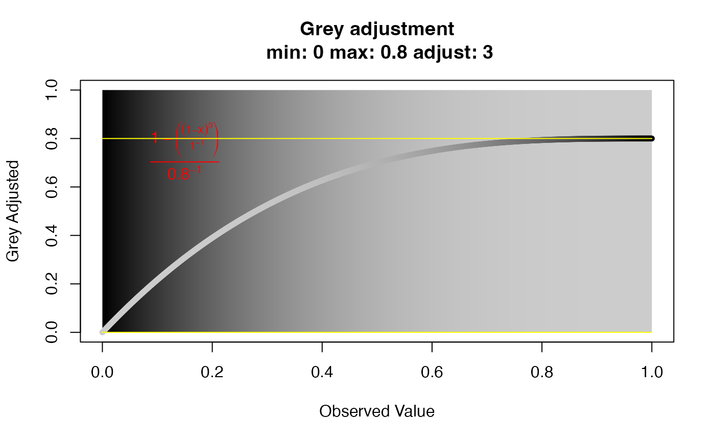
Display a greyscale gradient adjusted to specific parameters

This function has one purpose. It is for deciding the appropriate scaling for a grey palette to be used for edge weights of a minimum spanning network.

Usage

greycurve(
  data = seq(0, 1, length = 1000),
  glim = c(0, 0.8),
  gadj = 3,
  gweight = 1,
  scalebar = FALSE
)

Arguments

data

a sequence of numbers to be converted to greyscale.

glim

"grey limit". Two numbers between zero and one. They determine the upper and lower limits for the gray function. Default is 0 (black) and 0.8 (20% black).

gadj

"grey adjust". a positive integer greater than zero that will serve as the exponent to the edge weight to scale the grey value to represent that weight.

gweight

"grey weight". an integer. If it's 1, the grey scale will be weighted to emphasize the differences between closely related nodes. If it is 2, the grey scale will be weighted to emphasize the differences between more distantly related nodes.

scalebar

When this is set to TRUE, two scalebars will be plotted. The purpose of this is for adding a scale bar to minimum spanning networks produced in earlier versions of poppr.

Value

A plot displaying a grey gradient from 0.001 to 1 with minimum and maximum values displayed as yellow lines, and an equation for the correction displayed in red.

Author

Zhian N. Kamvar

Examples

# Normal grey curve with an adjustment of 3, an upper limit of 0.8, and
# weighted towards smaller values.
greycurve()

# \dontrun{
# 1:1 relationship grey curve.
greycurve(gadj=1, glim=1:0)


# Grey curve weighted towards larger values.
greycurve(gweight=2)


# Same as the first, but the limit is 1.
greycurve(glim=1:0)


# Setting the lower limit to 0.1 and weighting towards larger values.
greycurve(glim=c(0.1,0.8), gweight=2)

# }